dual multi-period excess earnings in the valuation … multi-period excess earnings in the valuation...

October 2013

Dual Multi-Period Excess Earnings in the Valuation of Intangibles

Copyright © 2013 American Institute of CPAs. All rights reserved.

DISCLAIMER: This publication has not been approved, disapproved or otherwise acted upon by any senior technical committees of and does not represent an official position of the American Institute of CPAs. It is distributed with the understanding that the AICPA is not rendering legal, accounting or other professional services in this publication. If legal advice or other expert assistance is required, the services of a competent professional should be sought.

For more information about the procedure for requesting permission to make copies of any part of this work, please email [email protected] with your request. Otherwise, requests should be written and mailed to the Permissions Department, AICPA, 220 Leigh Farm Road, Durham, NC 27707-8110.

ContRIbutIng AutHoRS:

Randie Dial Partner — CliftonLarsonAllen LLP

Carol Lewis Partner — BKD, LLP

Michael Massey Partner — Moss Adams LLP

Brian Steen Principal — Dixon Hughes Goodman LLP

REVIEwERS:

The Forensic and Valuation Services team and the authors thank the members of the 2012-13 AICPA Forensic and Valuation Services Executive Committee and AICPA Business Valuations Committee for reviewing this white paper.

tAbLE oF ContEntS

Executive Summary . . . . . . . . . . . . . . . . . . . . . . . . . . . . . . . . . . . . . . . . . . . . . . . . . . . . . . . . . . . . . . . . . . . . . . . . . . . . . . . . . . . . . . . . . . . . . . . . .2

Method overview . . . . . . . . . . . . . . . . . . . . . . . . . . . . . . . . . . . . . . . . . . . . . . . . . . . . . . . . . . . . . . . . . . . . . . . . . . . . . . . . . . . . . . . . . . . . . . . . . . .3

Hierarchy Method . . . . . . . . . . . . . . . . . . . . . . . . . . . . . . . . . . . . . . . . . . . . . . . . . . . . . . . . . . . . . . . . . . . . . . . . . . . . . . . . . . . . . . . . . . . . . . . . . . .4

Cross-Charge Method . . . . . . . . . . . . . . . . . . . . . . . . . . . . . . . . . . . . . . . . . . . . . . . . . . . . . . . . . . . . . . . . . . . . . . . . . . . . . . . . . . . . . . . . . . . . . .5

Partial Separation Method . . . . . . . . . . . . . . . . . . . . . . . . . . . . . . . . . . . . . . . . . . . . . . . . . . . . . . . . . . . . . . . . . . . . . . . . . . . . . . . . . . . . . . . .6

Separation Method . . . . . . . . . . . . . . . . . . . . . . . . . . . . . . . . . . . . . . . . . . . . . . . . . . . . . . . . . . . . . . . . . . . . . . . . . . . . . . . . . . . . . . . . . . . . . . . . .7

Conclusion . . . . . . . . . . . . . . . . . . . . . . . . . . . . . . . . . . . . . . . . . . . . . . . . . . . . . . . . . . . . . . . . . . . . . . . . . . . . . . . . . . . . . . . . . . . . . . . . . . . . . . . . . . . .8

Examples . . . . . . . . . . . . . . . . . . . . . . . . . . . . . . . . . . . . . . . . . . . . . . . . . . . . . . . . . . . . . . . . . . . . . . . . . . . . . . . . . . . . . . . . . . . . . . . . . . . . . . . . . . . . .9

ExECutIVE SuMMARy

The purpose of this technical white paper is to discuss the application and issues of the multi-period excess earnings method (“MPEEM”) when two intangible assets are being valued using this method. This method typically is used to value the most important asset(s), (i.e., primary asset(s)) while other methods are used to value assets that are more secondary. Typically, the method is utilized to value only one of the subject intangible assets. However, in certain situations the method may be considered appropriate for two intangible assets when the assets are of similar importance to the company. For example, this case could be made for a technology company where technology is a driving force for the company, but strong customer relationships are also very important.

This technical white paper will address the following related to utilizing the MPEEM for more than one intangible asset (dual excess earnings):

Provide an overview of the methods

Discuss options to consider with examples

Identify advantages and disadvantages

It is important to note that this technical white paper is informational only regarding the use of the MPEEM. It does not promote or criticize the use of the methods discussed. this paper is prepared merely to provide information to the valuation community regarding the methods and the potential pros and cons.

Dual Multi-Period Excess Earnings in the Valuation of Intangibles | 2

MEtHoD oVERVIEw

The MPEEM is a form of the income approach and is generally reserved for the primary intangible asset with the most direct relationship to the revenue and cash flow stream. Unlike the discounted cash flow (”DCF”) method, the MPEEM measures fair value by discounting only the expected future cash flows attributable to a single intangible asset. To determine the cash flows attributable to a single intangible asset, those cash flows must be isolated by deducting a charge for the use of all the operating assets that contribute to the value of that intangible asset. The charge for the use of the operating assets is called a contributory charge. A contributory charge is a form of economic rent for the use of assets in generating the expected cash flows. After deducting these charges, the remaining residual cash flows are assumed to be the cash flows attributable to the subject intangible asset.

When this method is used to value more than one intangible asset, the primary issues that surface are:

1. Separating the cash flows for the two intangible assets; and/or

2. Cross charging the intangible assets for the use of the other intangible assets.

Splitting Revenues — One method for estimating the value of two separate intangible assets is to isolate the revenues and cash flows for the two intangible assets. This method can be utilized when the assets have two distinct revenue sources and the intangible assets are not dependent upon each other. If this were the case, the calculations would not require a cross charge for the two intangible assets. Splitting revenues is not always as straight forward as it sounds. For example, how do you eliminate the overlap category “sales of current technology to current customers?” This can often be overlooked when splitting revenues.

Cross Contributory Charges — This issue relates to the concept of charging one of the intangible assets for the use of the other and vice versa. For example, servicing the customer relationships requires the use of technology; therefore, a contributory charge should be deducted from the customer relationships’ cash flow for the use of the technology and vice versa. One of the biggest issues with this approach is the circular relationship between the two calculations (i.e., the value of each intangible asset depends on the contributory charge of the other intangible asset). Opinions differ on the usefulness and reliability of this approach. Some believe the method results in reliable values, while others believe the method results in values that may be overstated.

These issues are included and addressed in this white paper through the presentation of four dual excess earnings methods that exist. These methods include the Hierarchy Method, the Cross-Charge Method, the Partial Separation Method and the Separation Method. Each of these methods is unique and has its own nuances on how to deal with the above issues. This white paper addresses each method below with examples as well as the pros and cons.


HIERARCHy MEtHoD

The Hierarchy Method assumes that a hierarchy, or order of importance, exists between the two primary intangible assets. Under this method, both intangible assets are valued using an MPEEM and a contributory asset charge from the primary intangible asset is applied to the secondary intangible asset. However, the primary intangible asset does not receive a contributory asset charge from the secondary intangible asset.

If there is no acquired in-process research and development (IPR&D) or backlog, the Hierarchy Method is a relatively simplistic method for valuing dual primary intangible assets. However, careful consideration must be given to the selection of a primary intangible asset. This selection is subjective in nature and has an impact on the value of the primary and secondary intangible assets. A factor that should be considered in identifying the primary intangible asset includes the buyer’s motivation for acquiring the intangible assets. A buyer typically is able to identify the primary intangible asset that motivated them to make the acquisition. The buyer’s motivations likely reflect those of a market participant buyer and may identify the primary intangible asset. Past experience may also help the appraiser to identify the primary intangible asset considering the nature of the intangible assets and which intangible assets typically have a higher value or a longer life.

Because a contributory asset charge from the primary intangible asset is applied to the secondary intangible asset, but no contributory asset charge from the secondary intangible asset is applied to the primary intangible asset, the Hierarchy Method naturally provides a higher value for the primary intangible asset and a lower value for the secondary intangible asset. This is a main reason why the selection between primary and secondary intangible assets is a very important decision. In addition, because profits are not split between the two intangible assets, profits may be double-counted, further contributing to the overvaluation of the primary intangible asset. Profits allocated to the two intangible assets will not reconcile with total company profits.

The Hierarchy Method has additional theoretical problems in that the value of the secondary intangible asset has no impact on the value of the primary intangible asset. In theory, the value of enabling intangible assets should impact the value of the primary intangible asset. In the Hierarchy Method, however, the primary intangible asset value impacts the value of the secondary intangible asset only.

This white paper provides a high-level example in the section titled “Examples — Hierarchy Method.” This example assumes that technology was deemed to be the primary intangible asset while customer relationships were deemed to be a secondary intangible asset. As presented on Exhibits 2A and 2B, both intangible assets are valued using the MPEEM, but only the secondary intangible asset (i.e., customer relationships) is being charged a contributory charge relating to the value of the primary intangible asset (i.e., technology). The contributory charge sheet (Exhibit 2C) shows the calculation of the charges and how they are calculated.

Because the primary asset, technology, is not burdened by a contributory asset charge relating to customer relationships, its value may be overstated, as explained above. This again illustrates that the determination of which intangible asset is primary or secondary is very important.

Because a contributory asset charge from the primary intangible asset is applied to the secondary intangible asset, but no contributory asset charge from the secondary intangible asset is applied to the primary intangible asset, the Hierarchy Method naturally provides a higher value for the primary intangible asset and a lower value for the secondary intangible asset.


CRoSS-CHARgE MEtHoD

Unlike the Hierarchy Method, the Cross-Charge Method does not require the identification of a primary and secondary intangible asset. Under the Cross-Charge Method, both intangible assets are valued using an MPEEM and a contributory asset charge from each intangible asset is assigned to the other intangible asset.

The Cross-Charge Method may result in a reasonable value conclusion if the proper cross-charge assumptions are included in the calculation. However, there are no guidelines regarding how cross charges should be calculated. This is a weakness because the Cross-Charge Method is based on a circular reference due to the cross charges that are applied to each intangible asset. Therefore, intangible asset values can vary widely depending on how the appraiser chooses to set up the cross charges. This issue becomes more complicated if the two intangible assets have significantly different lives because the selected revenue base typically impacts the contributory asset charge calculation.

In addition, the Cross-Charge Method does not segregate profits. As a result, the profits allocated to the two intangible assets will not reconcile to the company’s total profit. This can result in the over or under-statement of intangible asset values.

A high-level example is presented in the section of this white paper titled “Examples — Cross-Charge Method.” As presented on Exhibits 3A and 3B, both intangible assets are valued using the MPEEM, but in this instance, they are both charged for each other’s use. In the technology valuation on Exhibit 3A, there is a charge relating to the customer relationships. In addition, in the valuation of the customer relationships on Exhibit 3B, there is a charge relating to the technology.

Exhibit 3C illustrates the contributory asset charge determination and how the calculation works. The first step is to segregate the forecast into four buckets as presented. These buckets represent both existing and future technology revenue as well as both existing and future customer relationships revenue. The return on both technology and customers relationships is then determined by taking the discount rate applicable to each multiplied by their respective value. In Exhibit 3C, the value of the technology is presented as $1,756 and a discount rate of 16%. This implies a return of $281. This is why the analysis becomes circular as you have to know the “value” to determine the return required.

The valuation of IPR&D and backlog may result in additional circular references.

The Appraisal Foundation recommends that the Cross-Charge Method “is not best practice and should be avoided.”1

1 Best Practices for Valuations in Financial Reporting: Intangible Asset Working Group — Contributory Assets, May 31, 2010, The Appraisal Foundation

The Cross-Charge Method may result in a reasonable value conclusion if the proper cross charge assumptions are included in the calculation. However, there are no guidelines regarding how cross charges should be calculated.


PARtIAL SEPARAtIon MEtHoD

Under the Partial Separation Method, an MPEEM is applied to one intangible asset using a contributory asset charge for another intangible asset, the value of which is determined in a two-step process. This method is complex and is more easily demonstrated through the use of a specific scenario. (See Examples — Partial Separation Method.)

In this scenario, the company has technology and customer relationships. This method determines a contributory asset charge for the customer relationships by applying an MPEEM to the existing customers based on the future technology only (see Exhibit 4B). An MPEEM is also applied to the company’s existing technology (see Exhibit 4A). The contributory asset charge for customer relationships that was applied in the existing technology MPEEM is added to the customer relationships/future technology cash flows in order to arrive at total cash flows resulting from customer relationships (see Exhibit 4C). These cash flows drive the value of customer relationships and the contributory asset charge applied to existing technology.

A benefit of the Partial Separation Method is that it begins to separate cash flows between the two assets to be valued. However, the Partial Separation Method has a number of challenges. One challenge is that it contains a circular reference. The customer relationships contributory asset charge applied to existing technology is based the total value of existing customer relationships, which is based, in part, on the contributory asset charge applied to existing technology. Therefore, it results in a circular reference. In addition, some argue that business enterprise revenue basis of the customer relationships contributory asset charge calculation is subjective.

Similar to prior methodologies that we discussed in previous sections of this white paper, the profits allocated to the two assets will not reconcile to the company’s total profit.

Finally, the method does not separate existing technology revenues between existing and future customers. As a result, this methodology may overstate the value of existing customer relationships.

A high-level example is presented in the section of this white paper titled “Examples — Partial Separation Method.” Note that in the calculation of the value of customer relationships, Exhibit 4B (Step 2a), that the revenue reflects only the future technology sold to existing customers. The residual profit from Step 2a is added to the customer relationship CAC that is utilized in Exhibit 4A (Step 1) to determine the total value of customer relationships.

A benefit of the Partial Separation Method is that it begins to separate cash flows between the two assets to be valued. However, the Partial Separation Method has a number of challenges.


SEPARAtIon MEtHoD

Following the scenario discussed above (assuming technology and customer relationships), the last method gets even more complicated. Under the Separation Method, revenues are split between existing and future customers and technology. In addition, research and development expenses are split between existing and future technology and sales and marketing expenses are split between existing and future customers. The development and presentation of the revenue and expense splitting is referred to as Step 0 and is presented on Exhibits 5A and 5B. The value of the technology intangible asset and customer relationships intangible asset is then determined in a multi-step process as follows:

First, an MPEEM is applied to existing technology attributable to future customers on Exhibit 5C. In this analysis, only maintenance research and development, future sales and marketing expense, and general contributory asset charges are applied. This step provides one portion of the existing technology value. The existing technology royalty rate implied by the first calculation is calculated using the revenue stream attributable to existing technology and future customers (Exhibit 5D).

Second, an MPEEM is applied to existing technology and existing customers as presented on Exhibit 5E. In this analysis, maintenance research and development, maintenance sales and marketing, general contributory asset charges and a technology contributory asset charge (as determined by the royalty above) are applied to arrive at a portion of the customer relationships value. This step provides one portion of the customer relationships value.

Third, the present value of the technology contributory asset charge applied in the second step is calculated (Exhibit 5F). This step provides the second portion of the existing technology value.

Fourth, an MPEEM is applied to future technology and existing customers. In this analysis, future research and development, maintenance sales and marketing expenses and general contributory asset charges are applied to arrive at the second portion of the customer relationships value (Exhibit 5G).

Finally, the result of Steps 1 and 3 are added to arrive at existing technology value and the results of Steps 2 and 4 are added to arrive at the value of customer relationships.

A high-level example is presented in the section of this white paper titled “Examples — Separation Method.” Note that the separation map for revenue and expenses (Step 0) is included in Exhibits 5A and 5B, and that the total revenue reconciles to the revenue presented in the business enterprise value, Exhibit 1A. The conclusions of Steps 1 and 3 (for technology) and Steps 2 and 4 are (for customer relationships) presented in Exhibit 5H.

This separation of revenues and expenses enables the valuation of existing technology and existing customers without the use of circular references using profits that reconcile to the Company’s total profit. Therefore, it is believed it is more theoretically sound than the other methods described above.

Drawbacks of the Separation Method revolve around the complexity of mapping revenues and expenses between existing and future customers and technology. This process is further complicated if IPR&D or backlog is introduced into the valuation as additional revenue and expense maps must be built into the model.

If the existing technology is expected to generate different returns when sold to future customers compared to the returns generated from existing customers, adjustments may need to be applied to the implied royalty rate.


As presented in this paper, there are several methods to choose from in applying a dual excess earnings approach. These methods each have their benefits and drawbacks. In practice, most appraisers are able to find methods other than MPEEM to value one of the intangible assets in order to avoid using a dual excess earnings approach.

The examples are provided to give the reader a sense of how complex these methods can get. They often get very difficult reviews and questions because of the embedded assumptions and circular equations within the models. These examples were purely shown as hypothetical situations and are not meant to be copied and used. The narrative of this paper was meant to discuss these methods at a summary level to give the reader a sense of how the methods work and their difficulties. This paper was not meant to give the reader a roadmap of how to apply the methods, but was written at more of a demonstrative level.

In the end, it is the choice of the practitioner on which methods to ultimately employ and it is his/her responsibility to justify the decision.

ConCLuSIon


Examples for all the methods discussed above are presented in this section. The examples consider a technology industry company acquisition at the end of 2013 of about $16 million, where both the technology and the customer relationships were the primary value drivers of the transaction. Other important assumptions for the analysis are:

ExAMPLES

In addition, although the examples do not present the determination of the weighted average cost of capital, it was determined that 16% was the required rate of return for both the customer relationships and the technology. The determination of the business enterprise value is presented in Exhibit 1A (note that the internal rate of return determined in the business enterprise value analysis is 15.0%) and a mid-year convention is utilized.

Note that the conclusions under the various methods vary significantly. Under the Hierarchy Method, the technology value (it had been determined technology was the primary intangible asset) is much greater than the value determined in any of the other methods. The conclusions under the other methods are more closely aligned, as presented below.

Last year of technology 2018

Existing Customers Revenue growth percentage

2.00%

Customer Relationship Attrition each year

20.00%

Point when existing customers become less than 2% of sales

2025

Hierarchy Method technology $2,626

Customer Relationships $1,725

Cross-Charge Method technology $1,756


Partial Separation Method technology

$2,000


Separation Method technology $2,300



ExHIbIt 1A — DISCOUNTED CASH FLOW ANALYSIS – BUSINESS ENTERPRISE VALUE (BEV)

Most recent terminal 12 months 2014 2015 2016 2017 2018 2019 2020 2021 2022 2023 2024 Period

Net Revenue 12,500 15,000 17,500 18,500 19,000 19,500 20,000 20,500 21,000 21,500 22,000 22,500 23,000

Growth 20.00% 16.67% 5.71% 2.70% 2.63% 2.56% 2.50% 2.44% 2.38% 2.33% 2.27% 2.22%

Cost of Goods Sold 6,000 7,000 7,400 7,600 7,800 8,000 8,200 8,400 8,600 8,800 9,000 9,200

Gross Profit 9,000 10,500 11,100 11,400 11,700 12,000 12,300 12,600 12,900 13,200 13,500 13,800

60.00% 60.00% 60.00% 60.00% 60.00% 60.00% 60.00% 60.00% 60.00% 60.00% 60.00% 60.00%

R&D Expense 1,500 1,750 1,850 1,900 1,950 2,000 2,050 2,100 2,150 2,200 2,250 2,300

10.00% 10.00% 10.00% 10.00% 10.00% 10.00% 10.00% 10.00% 10.00% 10.00% 10.00% 10.00%

S&M Expense 2,250 2,625 2,775 2,850 2,925 3,000 3,075 3,150 3,225 3,300 3,375 3,450

15.00% 15.00% 15.00% 15.00% 15.00% 15.00% 15.00% 15.00% 15.00% 15.00% 15.00% 15.00%

G&A Expense 1,500 1,750 1,850 1,900 1,950 2,000 2,050 2,100 2,150 2,200 2,250 2,300

10.00% 10.00% 10.00% 10.00% 10.00% 10.00% 10.00% 10.00% 10.00% 10.00% 10.00% 10.00%

Total Operating Expenses 5,250 6,125 6,475 6,650 6,825 7,000 7,175 7,350 7,525 7,700 7,875 8,050

EBITDA 3,750 4,375 4,625 4,750 4,875 5,000 5,125 5,250 5,375 5,500 5,625 5,750

25.00% 25.00% 25.00% 25.00% 25.00% 25.00% 25.00% 25.00% 25.00% 25.00% 25.00% 25.00%

Depreciation 750 875 925 950 975 1,000 1,025 1,050 1,075 1,100 1,125 1,150

5.00% 5.00% 5.00% 5.00% 5.00% 5.00% 5.00% 5.00% 5.00% 5.00% 5.00% 5.00%

Operating Income 3,000 3,500 3,700 3,800 3,900 4,000 4,100 4,200 4,300 4,400 4,500 4,600

20.00% 20.00% 20.00% 20.00% 20.00% 20.00% 20.00% 20.00% 20.00% 20.00% 20.00% 20.00%

Tax Expense 40.00% 1,200 1,400 1,480 1,520 1,560 1,600 1,640 1,680 1,720 1,760 1,800 1,840

After-Tax Operating Income 1,800 2,100 2,220 2,280 2,340 2,400 2,460 2,520 2,580 2,640 2,700 2,760

Plus: Depreciation 750 875 925 950 975 1,000 1,025 1,050 1,075 1,100 1,125 1,150

Less: CapEx 6.00% (900) (1,050) (1,110) (1,140) (1,170) (1,200) (1,230) (1,260) (1,290) (1,320) (1,350) (1,150)

Less: Changes in debt-free Net Working Capital 10.00% (250) (250) (100) (50) (50) (50) (50) (50) (50) (50) (50) (50)

Unlevered Free Cash Flow 1,400 1,675 1,935 2,040 2,095 2,150 2,205 2,260 2,315 2,370 2,425 2,710

9.33% 9.57% 10.46% 10.74% 10.74% 10.75% 10.76% 10.76% 10.77% 10.77% 10.78% 11.78%

Partial Period Factor 1 1 1 1 1 1 1 1 1 1 1

Mid-Year Convention 0.5 1.5 2.5 3.5 4.5 5.5 6.5 7.5 8.5 9.5 10.5

Present Value Factor 15.00% 0.9325 0.8109 0.7051 0.6131 0.5332 0.4636 0.4031 0.3506 0.3048 0.2651 0.2305

Present Value of Cash Flow

Net Present Value of Discrete Cash Flows 1,306 1,358 1,364 1,251 1,117 997 889 792 706 628 559

Net Present Value of Residual Cash Flows 5,205

Purchase Price 16,172

Implied Multiple of 2011 EBITDA 4.31

Plus: Excess WC 0

Plus: NonOperating Assets, Net 0

Plus: NonOperating Loss Valuation 0

Total Consideration, Rounded 16,176

terminal Value

Residual Cash Flow 2,710

WACC 15.00%

Long-term Growth 3.00%

Divided by Cap Rate 12.00%

22,583

PV Factor 0.2305

5,205


ExHIbIt 2A — HIERARCHY METHOD – EXISTING TECHNOLOGY VALUE (PRIMARY ASSET) as of Dec. 31, 2013

2014 2015 2016 2017 2018

Existing Technology Revenue 12,000 9,600 6,720 4,032 2,016 Growth -20.00% -30.00% -40.00% -50.00%

Cost of Goods Sold 4,800 3,840 2,688 1,613 806

Gross Profit 7,200 5,760 4,032 2,419 1,210 60.00% 60.00% 60.00% 60.00% 60.00%

Maintenance/R&D Expense 1,200 960 672 403 202 10.00% 10.00% 10.00% 10.00% 10.00%

S&M Expense 1,800 1,440 1,008 605 302 15.00% 15.00% 15.00% 15.00% 15.00%

G&A Expense 1,200 960 672 403 202 10.00% 10.00% 10.00% 10.00% 10.00%

Total Operating Expenses 4,200 3,360 2,352 1,411 706

EBITDA 3,000 2,400 1,680 1,008 504 25.00% 25.00% 25.00% 25.00% 25.00%

Depreciation 600 480 336 202 101 5.00% 5.00% 5.00% 5.00% 5.00%

Operating Income 2,400 1,920 1,344 806 403 20.00% 20.00% 20.00% 20.00% 20.00%

Tax Expense 40.00% 960 768 538 323 161

After-Tax Operating Income 1,440 1,152 806 484 242

After-Tax Capital Charges Net Working Capital 0.60% 72 58 40 24 12 Fixed Assets 2.40% 288 230 161 97 48 Assembled Workforce 0.80% 96 77 54 32 16

456 365 255 153 77

Residual Profit 984 787 551 331 165 8.20% 8.20% 8.20% 8.20% 8.20%

Partial Period Factor 1 1 1 1 1 Mid-Year Convention 0.5 1.5 2.5 3.5 4.5 Present Value Factor 16.00% 0.9285 0.8004 0.6900 0.5948 0.5128 Present Value of Cash Flow

Net Present Value of Discrete Cash Flows 914 630 380 197 85

2,205 Tax Amortization Benefit 420 Fair Value of Developed technology 2,626


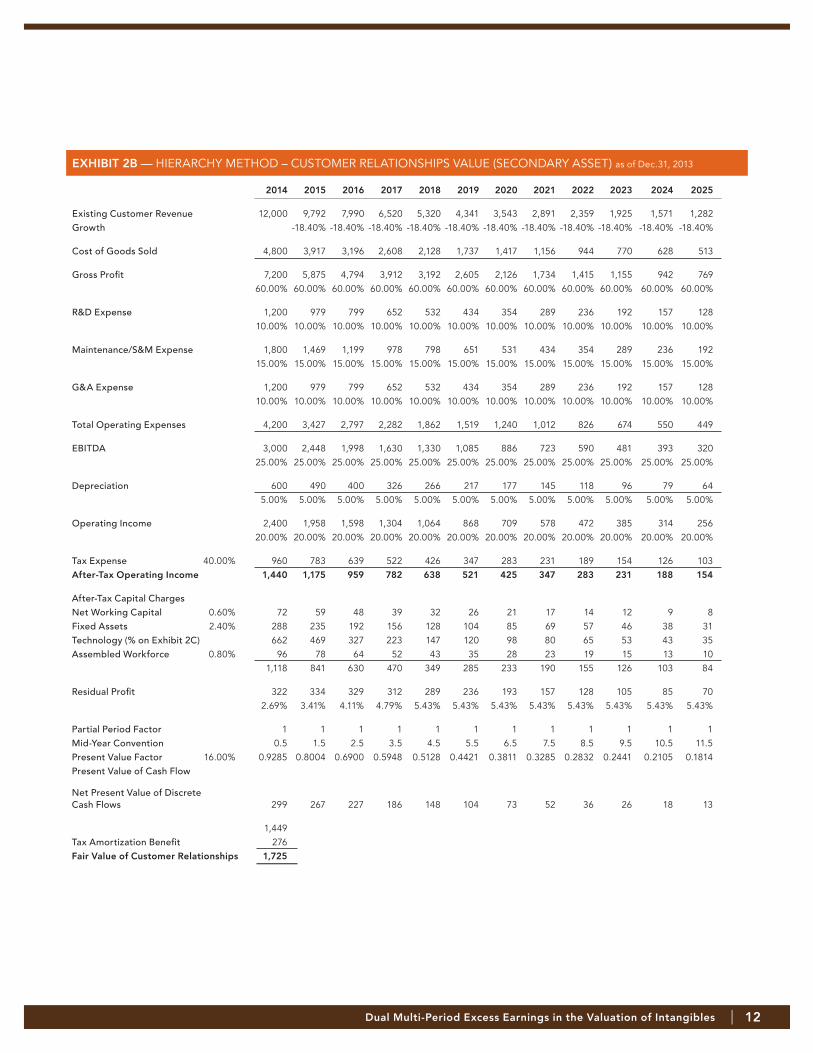
ExHIbIt 2b — HIERARCHY METHOD – CUSTOMER RELATIONSHIPS VALUE (SECONDARY ASSET) as of Dec.31, 2013

2014 2015 2016 2017 2018 2019 2020 2021 2022 2023 2024 2025

Existing Customer Revenue 12,000 9,792 7,990 6,520 5,320 4,341 3,543 2,891 2,359 1,925 1,571 1,282 Growth -18.40% -18.40% -18.40% -18.40% -18.40% -18.40% -18.40% -18.40% -18.40% -18.40% -18.40%

Cost of Goods Sold 4,800 3,917 3,196 2,608 2,128 1,737 1,417 1,156 944 770 628 513

Gross Profit 7,200 5,875 4,794 3,912 3,192 2,605 2,126 1,734 1,415 1,155 942 769 60.00% 60.00% 60.00% 60.00% 60.00% 60.00% 60.00% 60.00% 60.00% 60.00% 60.00% 60.00%

R&D Expense 1,200 979 799 652 532 434 354 289 236 192 157 128 10.00% 10.00% 10.00% 10.00% 10.00% 10.00% 10.00% 10.00% 10.00% 10.00% 10.00% 10.00%

Maintenance/S&M Expense 1,800 1,469 1,199 978 798 651 531 434 354 289 236 192 15.00% 15.00% 15.00% 15.00% 15.00% 15.00% 15.00% 15.00% 15.00% 15.00% 15.00% 15.00%

G&A Expense 1,200 979 799 652 532 434 354 289 236 192 157 128 10.00% 10.00% 10.00% 10.00% 10.00% 10.00% 10.00% 10.00% 10.00% 10.00% 10.00% 10.00%

Total Operating Expenses 4,200 3,427 2,797 2,282 1,862 1,519 1,240 1,012 826 674 550 449

EBITDA 3,000 2,448 1,998 1,630 1,330 1,085 886 723 590 481 393 320 25.00% 25.00% 25.00% 25.00% 25.00% 25.00% 25.00% 25.00% 25.00% 25.00% 25.00% 25.00%

Depreciation 600 490 400 326 266 217 177 145 118 96 79 64 5.00% 5.00% 5.00% 5.00% 5.00% 5.00% 5.00% 5.00% 5.00% 5.00% 5.00% 5.00%

Operating Income 2,400 1,958 1,598 1,304 1,064 868 709 578 472 385 314 256 20.00% 20.00% 20.00% 20.00% 20.00% 20.00% 20.00% 20.00% 20.00% 20.00% 20.00% 20.00%

Tax Expense 40.00% 960 783 639 522 426 347 283 231 189 154 126 103 After-tax operating Income 1,440 1,175 959 782 638 521 425 347 283 231 188 154

After-Tax Capital Charges Net Working Capital 0.60% 72 59 48 39 32 26 21 17 14 12 9 8 Fixed Assets 2.40% 288 235 192 156 128 104 85 69 57 46 38 31 Technology (% on Exhibit 2C) 662 469 327 223 147 120 98 80 65 53 43 35 Assembled Workforce 0.80% 96 78 64 52 43 35 28 23 19 15 13 10 1,118 841 630 470 349 285 233 190 155 126 103 84

Residual Profit 322 334 329 312 289 236 193 157 128 105 85 70 2.69% 3.41% 4.11% 4.79% 5.43% 5.43% 5.43% 5.43% 5.43% 5.43% 5.43% 5.43%

Partial Period Factor 1 1 1 1 1 1 1 1 1 1 1 1 Mid-Year Convention 0.5 1.5 2.5 3.5 4.5 5.5 6.5 7.5 8.5 9.5 10.5 11.5 Present Value Factor 16.00% 0.9285 0.8004 0.6900 0.5948 0.5128 0.4421 0.3811 0.3285 0.2832 0.2441 0.2105 0.1814 Present Value of Cash Flow

Net Present Value of Discrete Cash Flows 299 267 227 186 148 104 73 52 36 26 18 13

1,449 Tax Amortization Benefit 276

Fair Value of Customer Relationships 1,725


ExHIbIt 2C — HIERARCHY METHOD – TECHNOLOGY CAC CALCULATION

*** Several methods here to use in determining the primary asset CAC. The value of the secondary asset will change depending on the method used but the value of the primary asset will not change.

Value of Technology 2,626

Useful Life 5

Annual Amortization 525

Required Return on Technology 16.00%

Return oF, and Full Return on over bEV Revenue through Customer Life 2014 2015 2016 2017 2018 2019 2020 2021

Return OF Technology 525 525 525 525 525 0 0 0

Return ON Technology 420 420 420 420 420 420 420 420

Total BEV Revenues 15,000 17,500 18,500 19,000 19,500 20,000 20,500 21,000

Total Return On and OF Technology 6.30% 5.40% 5.11% 4.98% 4.85% 2.10% 2.05% 2.00%

Return on only over bEV Revenue 2014 2015 2016 2017 2018

Return OF Technology 0 0 0 0 0

Return ON Technology 420 420 420 420 420

Total BEV Revenues 15,000 17,500 18,500 19,000 19,500

Total Return On and OF Technology 2.80% 2.40% 2.27% 2.21% 2.15%

Return on only over bEV Revenue through Customer Life 2014 2015 2016 2017 2018 2019 2020 2021

Return OF Technology 0 0 0 0 0 0 0 0



Total Return On and OF Technology 2.80% 2.40% 2.27% 2.21% 2.15% 2.10% 2.05% 2.00%

Return oF, and Full Return on over bEV Revenue 2014 2015 2016 2017 2018



Total BEV Revenues 15,000 17,500 18,500 19,000 19,500

Total Return On and OF Technology 6.30% 5.40% 5.11% 4.98% 4.85%

After-tax Return oF, Amortizing Return on over Existing Customer Revenue 2014 2015 2016 2017 2018

Technology Amortization 525 525 525 525 525

Tax (210) (210) (210) (210) (210)


Technology Value at Year-End 2,101 1,576 1,050 525 0


Total Return On and OF Technology 735 651 567 483 399

Existing Customers Portion of Technology 90% 72% 58% 46% 37%

Total Technology CAC for Existing Customers 662 469 327 223 147

Existing Customers Revenues 12,000 9,792 7,990 6,520 5,320

Technology CAC 5.51% 4.79% 4.09% 3.41% 2.77%


ExHIbIt 3A — CROSS-CHARGE METHOD – ESTIMATE OF EXISTING TECHNOLOGY as of Dec. 31, 2013

2014 2015 2016 2017 2018

Existing Technology Revenue 12,000 9,600 6,720 4,032 2,016 Growth -20.00% -30.00% -40.00% -50.00%


Gross Profit 7,200 5,760 4,032 2,419 1,210 60.00% 60.00% 60.00% 60.00% 60.00%

Maintenance/R&D Expense 1,200 960 672 403 202 10.00% 10.00% 10.00% 10.00% 10.00%

S&M Expense 1,800 1,440 1,008 605 302 15.00% 15.00% 15.00% 15.00% 15.00%

G&A Expense 1,200 960 672 403 202 10.00% 10.00% 10.00% 10.00% 10.00%


EBITDA 3,000 2,400 1,680 1,008 504 25.00% 25.00% 25.00% 25.00% 25.00%

Depreciation 600 480 336 202 101 5.00% 5.00% 5.00% 5.00% 5.00%


Tax Expense 40.00% 960 768 538 323 161


After-Tax Capital Charges Net Working Capital 0.60% 72 58 40 24 12 Fixed Assets 2.40% 288 230 161 97 48 CUSTOMER RELATIONSHIPS (Exhibit 3C) 2.72% 326 261 183 110 55 Assembled Workforce 0.80% 96 77 54 32 16

782 626 438 263 131

Residual Profit 658 526 368 221 111 5.48% 5.48% 5.48% 5.48% 5.48%


Net Present Value of Discrete Cash Flows 611 421 254 131 57 1,475 Tax Amortization Benefit 281 Fair Value of Developed Technology 1,756


ExHIbIt 3b — CROSS-CHARGE METHOD – ESTIMATE OF CUSTOMER RELATIONSHIPS as of Dec. 31, 2013

2014 2015 2016 2017 2018 2019 2020 2021 2022 2023 2024 2025

Existing Customer Revenue 12,000 9,792 7,990 6,520 5,320 4,341 3,543 2,891 2,359 1,925 1,571 1,282 Growth -18.40% -18.40% -18.40% -18.40% -18.40% -18.40% -18.40% -18.40% -18.40% -18.40% -18.40%

Cost of Goods Sold 4,800 3,917 3,196 2,608 2,128 1,737 1,417 1,156 944 770 628 513

Gross Profit 7,200 5,875 4,794 3,912 3,192 2,605 2,126 1,734 1,415 1,155 942 769 60.00% 60.00% 60.00% 60.00% 60.00% 60.00% 60.00% 60.00% 60.00% 60.00% 60.00% 60.00%

R&D Expense 1,200 979 799 652 532 434 354 289 236 192 157 128 10.00% 10.00% 10.00% 10.00% 10.00% 10.00% 10.00% 10.00% 10.00% 10.00% 10.00% 10.00%

Maintenance/S&M Expense 1,800 1,469 1,199 978 798 651 531 434 354 289 236 192 15.00% 15.00% 15.00% 15.00% 15.00% 15.00% 15.00% 15.00% 15.00% 15.00% 15.00% 15.00%

G&A Expense 1,200 979 799 652 532 434 354 289 236 192 157 128 10.00% 10.00% 10.00% 10.00% 10.00% 10.00% 10.00% 10.00% 10.00% 10.00% 10.00% 10.00%

Total Operating Expenses 4,200 3,427 2,797 2,282 1,862 1,519 1,240 1,012 826 674 550 449

EBITDA 3,000 2,448 1,998 1,630 1,330 1,085 886 723 590 481 393 320 25.00% 25.00% 25.00% 25.00% 25.00% 25.00% 25.00% 25.00% 25.00% 25.00% 25.00% 25.00%

Depreciation 600 490 400 326 266 217 177 145 118 96 79 64 5.00% 5.00% 5.00% 5.00% 5.00% 5.00% 5.00% 5.00% 5.00% 5.00% 5.00% 5.00%

Operating Income 2,400 1,958 1,598 1,304 1,064 868 709 578 472 385 314 256 20.00% 20.00% 20.00% 20.00% 20.00% 20.00% 20.00% 20.00% 20.00% 20.00% 20.00% 20.00%

Tax Expense 40.00% 960 783 639 522 426 347 283 231 189 154 126 103

After-Tax Operating Income 1,440 1,175 959 782 638 521 425 347 283 231 188 154

After-Tax Capital Charges Net Working Capital 0.60% 72 59 48 39 32 26 21 17 14 12 9 8 Fixed Assets 2.40% 288 235 192 156 128 104 85 69 57 46 38 31 TECHNOLOGY 1.65% 198 162 132 108 88 72 58 48 39 32 26 21 Assembled Workforce 0.80% 96 78 64 52 43 35 28 23 19 15 13 10 654 534 435 355 290 237 193 158 129 105 86 70

Residual Profit 786 641 523 427 348 284 232 189 155 126 103 84 6.55% 6.55% 6.55% 6.55% 6.55% 6.55% 6.55% 6.55% 6.55% 6.55% 6.55% 6.55%

Partial Period Factor 1 1 1 1 1 1 1 1 1 1 1 1 Mid-Year Convention 0.5 1.5 2.5 3.5 4.5 5.5 6.5 7.5 8.5 9.5 10.5 11.5 Present Value Factor 16.00% 0.9285 0.8004 0.6900 0.5948 0.5128 0.4421 0.3811 0.3285 0.2832 0.2441 0.2105 0.1814 Present Value of Cash Flow

Net Present Value of Discrete Cash Flows 730 513 361 254 179 126 88 62 44 31 22 15

2,425 Tax Amortization Benefit 462 Fair Value of Customer Relationships 2,887


ExHIbIt 3C — CROSS-CHARGE METHOD – TECHNOLOGY CAC CALCULATION

Value of Technology 1,756

Useful Life 5



Return of Technology 281

Return on over Average bEV Revenue 2011 and 2016

Technology CAC 1.65%

Customers CAC 2.72%

0.0165

Value of Customer Relationships 2,887

Useful Life 13



Return on Customers 462

Average bEV Revenues 2014 2014 2015 2016 2017 2018 2019 2020 2021

Cumulative Average BEV Revenues 15,000 16,250 17,000 17,500 17,900 18,250 18,571 18,875


Technology CAC% of Revenues 1.87% 1.73% 1.65%** 1.61% 1.57% 1.54% 1.51% 1.49%

Return ON Customers 462 462 462 462 462 462 462 462

Customer Relationship CAC % of Revenues 3.08% 2.84% 2.72% 2.64% 2.58% 2.53% 2.49% 2.45%

2014 2015 2016 2017 2018 2019 2020 2021

Existing Technology to Existing Customers 9,792 6,991 4,021 1,685 0 0 0 0

Future Technology to Existing Customers 2,448 4,661 6,031 6,739 7,055 5,904 4,938 4,128

Existing Technology to Future Customers 2,208 3,509 3,379 2,115 0 0 0 0

Future Technology to Future Customers 552 2,339 5,069 8,461 12,445 14,096 15,562 16,872


** The level of CAC depends on the selected average BEV Revenue Base


ExHIbIt 4A — PARTIAL SEPARATION METHOD Estimate of Existing Technology, Step 1

2014 2015 2016 2017 2018

Net Revenue 12,000 9,600 6,720 4,032 2,016 Growth n/a -20.00% -30.00% -40.00% -50.00%


Gross Profit 7,200 5,760 4,032 2,419 1,210 60.00% 60.00% 60.00% 60.00% 60.00%

Maintenance R&D Expense 1,200 960 672 403 202 10.00% 10.00% 10.00% 10.00% 10.00%

S&M Expense 1,800 1,440 1,008 605 302 15.00% 15.00% 15.00% 15.00% 15.00%

G&A Expense 1,200 960 672 403 202 10.00% 10.00% 10.00% 10.00% 10.00%


EBITDA 3,000 2,400 1,680 1,008 504 25.00% 25.00% 25.00% 25.00% 25.00%

Depreciation 600 480 336 202 101 5.00% 5.00% 5.00% 5.00% 5.00%


Tax Expense 40.00% 960 768 538 323 161


After Tax Capital Charges Net Working Capital 0.60% 72 58 40 24 12 Fixed Assets 2.40% 288 230 161 97 48 Customer Relationships 2.00% 240 192 134 81 40 Assembled Workforce 0.80% 96 77 54 32 16 Total Capital Charges 696 557 390 234 117

Residual Profit 744 595 417 250 125 6.20% 6.20% 6.20% 6.20% 6.20%


Net Present Value of Residual Profit 691 476 287 149 64 Sum of Residual Profit 1,667 Tax Amortization Benefit 318 Estimate of Developed Technology Fair Value 1,985

Estimate of Developed Technology Fair Value, Rounded 2,000


ExHIbIt 4b — PARTIAL SEPARATION METHOD Estimate of Existing Customer Relationships, Step 2A

2014 2015 2016 2017 2018 2019 2020 2021 2022

Net Revenue (Future Tech to Exist Cust) 2,400 4,420 5,088 5,136 4,770 4,341 3,543 2,891 2,359

Growth n/a 84.18% 15.10% 0.95% -7.13% -8.99% -18.40% -18.40% -18.40%

Less: Revenue Valued as Backlog - - - - - - - - -

Cost of Goods Sold 960 1,768 2,035 2,055 1,908 1,737 1,417 1,156 944

Gross Profit 1,440 2,652 3,053 3,082 2,862 2,605 2,126 1,734 1,415

60.00% 60.00% 60.00% 60.00% 60.00% 60.00% 60.00% 60.00% 60.00%

Future Technology R&D Expense 240 442 509 514 477 434 354 289 236

10.00% 10.00% 10.00% 10.00% 10.00% 10.00% 10.00% 10.00% 10.00%

Maintenance S&M Expense 360 884 1,018 1,027 954 868 709 578 472

15.00% 20.00% 20.00% 20.00% 20.00% 20.00% 20.00% 20.00% 20.00%

G&A Expense 240 442 509 514 477 434 354 289 236

10.00% 10.00% 10.00% 10.00% 10.00% 10.00% 10.00% 10.00% 10.00%

Total Operating Expenses 840 1,768 2,035 2,055 1,908 1,737 1,417 1,156 944

EBITDA 600 884 1,018 1,027 954 868 709 578 472

25.00% 20.00% 20.00% 20.00% 20.00% 20.00% 20.00% 20.00% 20.00%

Depreciation 120 221 254 257 239 217 177 145 118

5.00% 5.00% 5.00% 5.00% 5.00% 5.00% 5.00% 5.00% 5.00%

Operating Income 480 663 763 770 716 651 531 434 354

20.00% 15.00% 15.00% 15.00% 15.00% 15.00% 15.00% 15.00% 15.00%

Tax Expense 40.00% 192 265 305 308 286 260 213 173 142

After-Tax Operating Income 288 398 458 462 429 391 319 260 212

After Tax Capital Charges

Net Working Capital 0.60% 14 27 31 31 29 26 21 17 14

Fixed Assets 2.40% 58 106 122 123 114 104 85 69 57

Technology (Return ON only) 2.50% 60 111 127 128 119 109 89 72 59

Assembled Workforce 0.80% 19 35 41 41 38 35 28 23 19

Total Capital Charges 151 278 321 324 301 274 223 182 149

Residual Profit Net of Customer CAC

from Technology 137 119 137 139 129 117 96 78 64

5.70% 2.70% 2.70% 2.70% 2.70% 2.70% 2.70% 2.70% 2.70%


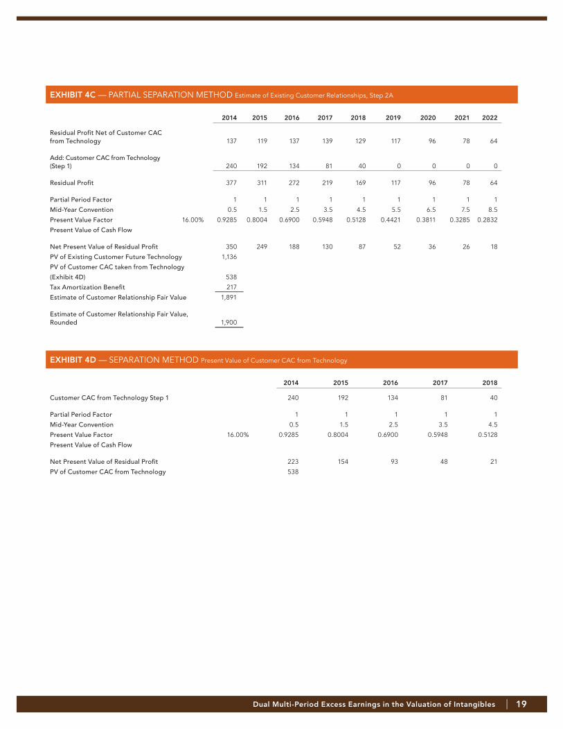
ExHIbIt 4C — PARTIAL SEPARATION METHOD Estimate of Existing Customer Relationships, Step 2A

ExHIbIt 4D — SEPARATION METHOD Present Value of Customer CAC from Technology

2014 2015 2016 2017 2018 2019 2020 2021 2022

Residual Profit Net of Customer CAC from Technology 137 119 137 139 129 117 96 78 64

Add: Customer CAC from Technology (Step 1) 240 192 134 81 40 0 0 0 0

Residual Profit 377 311 272 219 169 117 96 78 64

Partial Period Factor 1 1 1 1 1 1 1 1 1

Mid-Year Convention 0.5 1.5 2.5 3.5 4.5 5.5 6.5 7.5 8.5

Present Value Factor 16.00% 0.9285 0.8004 0.6900 0.5948 0.5128 0.4421 0.3811 0.3285 0.2832


Net Present Value of Residual Profit 350 249 188 130 87 52 36 26 18

PV of Existing Customer Future Technology 1,136

PV of Customer CAC taken from Technology

(Exhibit 4D) 538

Tax Amortization Benefit 217

Estimate of Customer Relationship Fair Value 1,891

Estimate of Customer Relationship Fair Value, Rounded 1,900

2014 2015 2016 2017 2018

Customer CAC from Technology Step 1 240 192 134 81 40

Partial Period Factor 1 1 1 1 1

Mid-Year Convention 0.5 1.5 2.5 3.5 4.5

Present Value Factor 16.00% 0.9285 0.8004 0.6900 0.5948 0.5128


Net Present Value of Residual Profit 223 154 93 48 21

PV of Customer CAC from Technology 538


ExHIbIt 5A — SEPARATION METHOD Dual Excess Earnings Method Revenue and Expense Map, Step 0

technology 2014 2015 2016 2017 2018 2019 2020 2021 2022

Existing Technology 12,000 9,600 6,720 4,032 2,016 - - - - % of Total 80.0% 54.9% 36.3% 21.2% 10.3% 0.0% 0.0% 0.0% 0.0%

Future Technology 3,000 7,900 11,780 14,968 17,484 20,000 20,500 21,000 21,500 % of Total 20.0% 45.1% 63.7% 78.8% 89.7% 100.0% 100.0% 100.0% 100.0%

Total Technology 15,000 17,500 18,500 19,000 19,500 20,000 20,500 21,000 21,500 % of BEV Revenue 100% 100% 100% 100% 100% 100% 100% 100% 100%

DEEM Revenue Map 2014 2015 2016 2017 2018 2019 2020 2021 2022

Existing Technology to Existing Customers 9,600 5,372 2,902 1,384 550 - - - - Future Technology to Existing Customers 2,400 4,420 5,088 5,136 4,770 4,341 3,543 2,891 2,359 Existing Technology to Future Customers 2,400 4,228 3,818 2,648 1,466 - - - - Future Technology to Future Customers 600 3,480 6,692 9,832 12,714 15,659 16,957 18,109 19,141 Total Revenue 15,000 17,500 18,500 19,000 19,500 20,000 20,500 21,000 21,500 % of BEV Revenue 100% 100% 100% 100% 100% 100% 100% 100% 100%

total bEV Revenue 15,000 17,500 18,500 19,000 19,500 20,000 20,500 21,000 21,500

Revenue Map

Customers 2014 2015 2016 2017 2018 2019 2020 2021 2022

Existing Customers 12,000 9,792 7,990 6,520 5,320 4,341 3,543 2,891 2,359 % of Total 80.0% 56.0% 43.2% 34.3% 27.3% 21.7% 17.3% 13.8% 11.0%

Future Customers 3,000 7,708 10,510 12,480 14,180 15,659 16,957 18,109 19,141 % of Total 20.0% 44.0% 56.8% 65.7% 72.7% 78.3% 82.7% 86.2% 89.0%

Total Customers 15,000 17,500 18,500 19,000 19,500 20,000 20,500 21,000 21,500 % of BEV Revenue 100% 100% 100% 100% 100% 100% 100% 100% 100%

ExHIbIt 5b — SEPARATION METHOD Dual Excess Earnings Method Revenue and Expense Map, Step 0

Sales & Marketing 2014 2015 2016 2017 2018 2019 2020 2021 2022

Existing Customers Maintenance S&M 1,800 1,958 1,598 1,304 1,064 868 709 578 472 % of Revenue 15.0% 20.0% 20.0% 20.0% 20.0% 20.0% 20.0% 20.0% 20.0%

Future Customers S&M 450 667 1,177 1,546 1,861 2,132 2,366 2,572 2,753 % of Revenue 15.0% 8.6% 11.2% 12.4% 13.1% 13.6% 14.0% 14.2% 14.4%

Total BEV S&M Expense 2,250 2,625 2,775 2,850 2,925 3,000 3,075 3,150 3,225 % of Revenue 15% 15% 15% 15% 15% 15% 15% 15% 15%

total bEV Revenue 15,000 17,500 18,500 19,000 19,500 20,000 20,500 21,000 21,500

Expense Map

Research & Development 2014 2015 2016 2017 2018 2019 2020 2021 2022

Existing Technology Maintenance R&D 1,200 720 336 121 - - - - - % of Revenue 10.0% 7.5% 5.0% 3.0% 0.0% 0.0% 0.0% 0.0% 0.0%

Future Technology R&D 300 1,030 1,514 1,779 1,950 2,000 2,050 2,100 2,150 % of Revenue 10.0% 13.0% 12.9% 11.9% 11.2% 10.0% 10.0% 10.0% 10.0%

Total BEV R&D Expense 1,500 1,750 1,850 1,900 1,950 2,000 2,050 2,100 2,150 % of Revenue 10% 10% 10% 10% 10% 10% 10% 10% 10%


ExHIbIt 5C — SEPARATION METHOD Estimate of Existing Technology to Future Customers, Step 1

2014 2015 2016 2017 2018

Net Revenue 2,400 4,228 3,818 2,648 1,466 Growth n/a 76.18% -9.72% -30.63% -44.65%

Cost of Goods Sold 960 1,691 1,527 1,059 586

Gross Profit 1,440 2,537 2,291 1,589 880 60.00% 60.00% 60.00% 60.00% 60.00%

Maintenance R&D Expense 240 423 382 265 147 10.00% 10.00% 10.00% 10.00% 10.00%

S&M Expense 360 366 428 328 192 15.00% 8.65% 11.20% 12.39% 13.12%

G&A Expense 240 423 382 265 147 10.00% 10.00% 10.00% 10.00% 10.00%

Total Operating Expenses 840 1,211 1,191 858 486

EBITDA 600 1,326 1,100 731 394 25.00% 31.35% 28.80% 27.61% 26.88%

Depreciation 120 211 191 132 73 5.00% 5.00% 5.00% 5.00% 5.00%

Operating Income 480 1,114 909 599 321 20.00% 26.35% 23.80% 22.61% 21.88%

Tax Expense 40.00% 192 446 363 240 128

After-Tax Operating Income 288 669 545 359 192

After Tax Capital Charges Net Working Capital 0.60% 14 25 23 16 9 Fixed Assets 2.40% 58 101 92 64 35 Assembled Workforce 0.80% 19 34 31 21 12 Total Capital Charges 91 161 145 101 56

Residual Profit 197 508 400 259 137 8.20% 12.01% 10.48% 9.77% 9.33%


Net Present Value of Residual Profit 183 407 276 154 70 Sum of Residual Profit 1,089 Tax Amortization Benefit 208 Estimate of Developed Technology Fair Value 1,297 Estimate of Developed Technology Fair Value, Rounded 1,300

ExHIbIt 5D — SEPARATION METHOD Estimate of Existing Technology to Future Customers, Step 1a

2014 2015 2016 2017 2018 2019 2020 2021 2022

Net Revenue 2,400 4,420 5,088 5,136 4,770 4,341 3,543 2,891 2,359 Growth n/a 84.18% 15.10% 0.95% -7.13% -8.99% -18.40% -18.40% -18.40%

Royalty Rate 9.00% 9.00% 9.00% 9.00% 9.00% 9.00% 9.00% 9.00% 9.00% 9.00%

Pretax Royalties 216 398 458 462 429 391 319 260 212

Tax Expense 40.00% 86 159 183 185 172 156 128 104 85

After-Tax Royalties 130 239 275 277 258 234 191 156 127

Partial Period Factor 1 1 1 1 1 1 1 1 1 Mid-Year Convention 0.5 1.5 2.5 3.5 4.5 5.5 6.5 7.5 8.5 Present Value Factor 16.00% 0.9285 0.8004 0.6900 0.5948 0.5128 0.4421 0.3811 0.3285 0.2832 Present Value of Cash Flow

Net Present Value of Residual Profit 120 191 190 165 132 104 73 51 36 Sum of Residual Profit 1,062 Tax Amortization Benefit 202 Estimate of Developed Technology Fair Value 1,264 Estimate of Developed Technology Fair Value, Rounded 1,300


ExHIbIt 5E — SEPARATION METHOD Estimate of Existing Customer Relationships from Existing Technology, Step 2

2014 2015 2016 2017 2018

Net Revenue 9,600 5,372 2,902 1,384 550 Growth n/a -44.05% -45.97% -52.33% -60.25%

Cost of Goods Sold 3,840 2,149 1,161 553 220

Gross Profit 5,760 3,223 1,741 830 330 60.00% 60.00% 60.00% 60.00% 60.00%

Maintenance R&D Expense 960 537 290 138 55 10.00% 10.00% 10.00% 10.00% 10.00%

Maintenance S&M Expense 1,440 1,074 580 277 110 15.00% 20.00% 20.00% 20.00% 20.00%

G&A Expense 960 537 290 138 55 10.00% 10.00% 10.00% 10.00% 10.00%

Total Operating Expenses 3,360 2,149 1,161 553 220

EBITDA 2,400 1,074 580 277 110 25.00% 20.00% 20.00% 20.00% 20.00%

Depreciation 480 269 145 69 28 5.00% 5.00% 5.00% 5.00% 5.00%

Operating Income 1,920 806 435 208 83 20.00% 15.00% 15.00% 15.00% 15.00%

Tax Expense 40.00% 768 322 174 83 33

After-Tax Operating Income 1,152 483 261 125 50

After Tax Capital Charges Net Working Capital 0.60% 58 32 17 8 3 Fixed Assets 2.40% 230 129 70 33 13 Technology 5.40% 518 290 157 75 30 Assembled Workforce 0.80% 77 43 23 11 4 Total Capital Charges 883 494 267 127 51

Residual Profit 269 (11) (6) (3) (1) 2.80% -0.20% -0.20% -0.20% -0.20%


Net Present Value of Residual Profit 250 (9) (4) (2) (1) Sum of Residual Profit 235 Tax Amortization Benefit 45 Estimate of Customer Relationship Fair Value 280

Estimate of Customer Relationship Fair Value, Rounded 300

ExHIbIt 5F — SEPARATION METHOD Estimate of Existing Technology to Existing Customers, Step 3

2014 2015 2016 2017 2018

After-Tax Royalties 518 290 157 75 30


Net Present Value of Residual Profit 481 232 108 44 15 Sum of Residual Profit 881 Tax Amortization Benefit 168 Estimate of Existing Technology to Existing Customers, 1,049

Estimate of Existing Technology to Existing Customers, Rounded 1,000


ExHIbIt 5g — SEPARATION METHOD Estimate of Existing Customers Buying Future Technology, Step 4

2014 2015 2016 2017 2018 2019 2020 2021 2022

Net Revenue 2,400 4,420 5,088 5,136 4,770 4,341 3,543 2,891 2,359 Growth n/a 84.18% 15.10% 0.95% -7.13% -8.99% -18.40% -18.40% -18.40%

Less: Revenue Valued as Backlog - - - - - - - - - Cost of Goods Sold 960 1,768 2,035 2,055 1,908 1,737 1,417 1,156 944

Gross Profit 1,440 2,652 3,053 3,082 2,862 2,605 2,126 1,734 1,415 60.00% 60.00% 60.00% 60.00% 60.00% 60.00% 60.00% 60.00% 60.00%

Future Technology R&D Expense 240 576 654 610 532 434 354 289 236 10.00% 13.04% 12.85% 11.89% 11.15% 10.00% 10.00% 10.00% 10.00%

Maintenance S&M Expense 360 884 1,018 1,027 954 868 709 578 472 15.00% 20.00% 20.00% 20.00% 20.00% 20.00% 20.00% 20.00% 20.00%

G&A Expense 240 442 509 514 477 434 354 289 236 10.00% 10.00% 10.00% 10.00% 10.00% 10.00% 10.00% 10.00% 10.00%

Total Operating Expenses 840 1,902 2,180 2,151 1,963 1,737 1,417 1,156 944

EBITDA 600 750 872 930 899 868 709 578 472 41.67% 28.27% 28.58% 30.19% 31.41% 33.33% 33.33% 33.33% 33.33%

Depreciation 120 221 254 257 239 217 177 145 118 5.00% 5.00% 5.00% 5.00% 5.00% 5.00% 5.00% 5.00% 5.00%

Operating Income 480 529 618 674 661 651 531 434 354 20.00% 11.96% 12.15% 13.11% 13.85% 15.00% 15.00% 15.00% 15.00%

Tax Expense 40.00% 192 212 247 269 264 260 213 173 142

After-Tax Operating Income 288 317 371 404 396 391 319 260 212

After Tax Capital Charges Net Working Capital 0.60% 14 27 31 31 29 26 21 17 14 Fixed Assets 2.40% 58 106 122 123 114 104 85 69 57 Technology 0.00% - - - - - - - - - Assembled Workforce 0.80% 19 35 41 41 38 35 28 23 19 Total Capital Charges 91 168 193 195 181 165 135 110 90

Residual Profit 197 149 177 209 215 226 184 150 123 8.20% 3.38% 3.49% 4.07% 4.51% 5.20% 5.20% 5.20% 5.20%

Partial Period Factor 1 1 1 1 1 1 1 1 1 Mid-Year Convention 0.5 1.5 2.5 3.5 4.5 5.5 6.5 7.5 8.5 Present Value Factor 16.00% 0.9285 0.8004 0.6900 0.5948 0.5128 0.4421 0.3811 0.3285 0.2832 Present Value of Cash Flow

Net Present Value of Residual Profit 183 119 122 124 110 100 70 49 35 Sum of Residual Profit 913 Tax Amortization Benefit 174 Estimate of Customer Relationship Fair Value 1,087

Estimate of Customer Relationship Fair Value, Rounded 1,100

ExHIbIt 5H — SEPARATION METHOD CONCLUSION OF FAIR VALUES

Customer Value

Step 2 300

Step 4 1,100

$ 1,400

Technology Value

Step 1 1,300

Step 3 1,000

$ 2,300


dual multi-period excess earnings in the valuation … multi-period excess earnings in the valuation...

Documents