improved t line contingency analysis in power … · system is essential for contingency analysis...

International Journal of Advances in Engineering & Technology, Nov. 2013.

©IJAET ISSN: 22311963

2159 Vol. 6, Issue 5, pp. 2159-2170

IMPROVED TRANSMISSION LINE CONTINGENCY ANALYSIS

IN POWER SYSTEM USING FAST DECOUPLED LOAD FLOW

Amit Kumar Roy1, Sanjay Kumar Jain2 1Asst.Professor, Department of Electrical Engineering,

JSS Academy of Technical Education, Noida, India 2Associate Professor, Department of Electrical & Instrumentation Engineering,

Thapar University, Patiala, India

ABSTRACT

Contingency analysis technique is being widely used to predict the effect of outages in power systems, like

failures of equipment, transmission line etc. The off line analysis to predict the effect of individual contingency

is a tedious task as a power system contains large number of components. Practically, only selected

contingencies will lead to severe conditions in power system like violation of voltage and active power flow

limits. The process of identifying these severe contingencies is referred as contingency selection and this can be

done by calculating performance indices for each contingencies. In this paper, the contingency selection by

calculating two kinds of performance indices; active power performance index (PIP) and reactive power

performance index (PIV) for single transmission line outage have been done with the help of Fast Decoupled

Load Flow (FDLF) in MATLAB environment. The ranking of most severe contingency has been done based on

the values of performance indices. Simultaneously the value of bus voltages and active power flow before and

after the most severe transmission line contingency has been analyzed. The effectiveness of the method has been

tested on 5-Bus, IEEE-14 Bus and IEEE-30 Bus test systems. It can be seen from the results that, based on the

knowledge of PIP & PIV the most severe transmission line contingency can be identified and the effect of this

contingency on the rest of the system can also be seen via post contingency analysis.

KEYWORDS: Contingency, contingency selection, performance indices, fast decoupled load flow.

I. INTRODUCTION

It is well known that power system is a complex network consisting of numerous equipments like

generators, transformers, transmission lines, circuit breakers etc. Failure of any of these equipments

during its operation harms the reliability of the system and hence leading to outages. Whenever the

pre specified operating limits of the power system gets violated the system is said to be in emergency

condition. These violations of the limits result from contingencies occurring in the system. Thus, an

important part of the security analysis revolves around the power system to withstand the effect of

contingencies. The contingency analysis is time consuming as it involves the computation of complete

AC load flow calculations following every possible outage events like outages occurring at various

generators and transmission lines. This makes the list of various contingency cases very lengthy and

the process very tedious. In order to mitigate the above problem, automatic contingency screening

approach is being adopted which identifies and ranks only those outages which actually causes the

limit violation on power flow or voltages in the lines. The contingencies are screened according to the

severity index or performance index where a higher value of these indices denotes a higher degree of

severity. The importance of power system security assessment for prediction of line flows and bus

voltages following a contingency has been presented in [1-2]. The paper also details the challenges

faced for the practical implementation of security analysis algorithms. The approximate changes in

the line flow due to an outage in generator or transmission line is predicted based on distribution

factors [3-4]. The use of AC power flow solution in outage studies has been dealt in [5].Contingency

screening or contingency selection is an essential task in contingency analysis. This helps to reduce



2160 Vol. 6, Issue 5, pp. 2159-2170

the numerous computations; the bounding method [6] reduces the number of branch flow computation

by using a bounding criterion that helps in reducing the number of buses for analysis and is based on

incremental angle criterion. The 1P-1Q method for contingency selection has been presented in [7]. In

this method the solution procedure is interrupted after an iteration of fast decoupled load flow.

Zaborzky et al. introduced the concentric relaxation method for contingency evaluation [8] utilizing

the benefit of the fact that an outage occurring on the power system has a limited geographical effect.

The use of fast decoupled load flow [9] proves to be very suitable for contingency analysis.

Contingency selection criterion based on the calculation of performance indices has been first

introduced by Ejebe and Wollenberg [10] where the contingencies are sorted in descending order of

the values of performance index (PI) reflecting their severity. The practical implementation of

contingency screening can be done by installing the phasor measurement units which are being used

to capture the online values of bus voltages and angles [11]. The fast estimation of voltages in power

system is essential for contingency analysis and this was proposed in [12]. Apart from performance

index other index like voltage stability criteria index can also be chosen contingency ranking [13].

Multiple contingency can occur in the power system at the same time, hence its identification and

analysis is a more complicated task, the multiple contingency screening in power system has been

illustrated in [14]. The analysis of power system contingency becomes more challenging when the

system is connected to a variable generation units like wind or solar systems, where the firm capacity

is variable. In [15] the contingency analysis by incorporating sampling of Injected powers has been

done.

In this paper, the values of active power performance index (PIP) and reactive power performance

index (PIV) have been calculated for 5-bus, IEEE-14 bus and IEEE-30 bus systems using the

algorithm implemented in MATLAB software. Based on the values of PIV, contingencies have been

ranked where a transmission line contingency leading to high value of PIV has been ranked 1 and a

least value of PIV have been ranked last. The load flow analysis following the most severe

transmission line contingency has been simulated and the results of active power flow in various

transmission lines and the bus voltages has been analyzed.

II. CONTINGENCY ANALYSIS USING LOAD FLOW SOLUTION

2.1 Contingency Selection

Since contingency analysis process involves the prediction of the effect of individual contingency

cases, the above process becomes very tedious and time consuming when the power system network

is large. In order to alleviate the above problem contingency screening or contingency selection

process is used. Practically it is found that all the possible outages does not cause the overloads or

under voltage in the other power system equipments. The process of identifying the contingencies that

actually leads to the violation of the operational limits is known as contingency selection. The

contingencies are selected by calculating a kind of severity indices known as Performance Indices (PI)

[1]. These indices are calculated using the conventional power flow algorithms for individual

contingencies in an off line mode. Based on the values obtained the contingencies are ranked in a

manner where the highest value of PI is ranked first. The analysis is then done starting from the

contingency that is ranked one and is continued till no severe contingencies are found. There are two

kind of performance index which are of great use, these are active power performance index (PIP) and

reactive power performance index (PIV). PIP reflects the violation of line active power flow and is

given by (1)

PIP = ∑ (Pi

Pimax)2nL

i=1 (1)

where,

Pi = Active Power flow in line i,

Pimax = Maximum active power flow in line i,

n is the specified exponent,

L is the total number of transmission lines in the system.



2161 Vol. 6, Issue 5, pp. 2159-2170

If n is a large number, the PI will be a small number if all flows are within limit, and it will be large if

one or more lines are overloaded, here the value of n has been kept unity. The value of maximum

power flow in each line is calculated using the formula

Pimax =

Vi∗Vj

𝑋 (2) where,

Vi= Voltage at bus i obtained from FDLF solution

Vj= Voltage at bus j obtained from FDLF solution

X = Reactance of the line connecting bus ‘i’ and bus ‘j’

Another performance index parameter which is used is reactive power performance index

corresponding to bus voltage magnitude violations. It mathematically given by (3)

PIV=∑ [2(𝑉𝑖−𝑉𝑖𝑛𝑜𝑚)

𝑉𝑖𝑚𝑎𝑥−𝑉𝑖𝑚𝑖𝑛]2𝑁𝑝𝑞

𝑖=1 (3)

where, Vi= Voltage of bus i, Vimax and Vimin are maximum and minimum voltage limits, Vinom is

average of Vimax and Vimin, Npq is total number of load buses in the system.

III. ALGORITHM FOR CONTINGENCY ANALYSIS USING FAST DECOUPLED

LOAD FLOW

The AC power flow program for contingency analysis by the Fast Decoupled Power Flow (FDLF) [9]

provides a fast solution to the contingency analysis since it has the advantage of matrix alteration

formula that can be incorporated and can be used to simulate the problem of contingencies involving

transmission line outages without re inverting the system Jacobian matrix for all iterations.

Set the contingency

counter K=0

Start

Simulate the line

outage contingency

Calculate the MW flows in all

the transmission line and PMax

using FDLF

Calculate the voltage at all

the buses using FDLF

Calculate PIP using (1)

Calculate PIV

using (2)

Last

contingency

reached ?

Increment the counter

K=K+1

Stop

Yes

No

Rank the contingencies as per

the highest value of PIP & PI

V

Read the system bus

data and line data

Do the power flow analysis for

the most severe contingency case

Print the results

Start

Read Bus Data

&

Line Data

Formulate the YBus

matrix of the system

and set counter K=0

(0) (0) (0)| | 1.0 0 0

i i iSet and for PQ bus and for PV busV

Calculate| |

P

V

?Does P converge?

Does Q

converge

Calculate' 1[ ]

| |

P

VB

Calculate| |

Q

V

?Does P converge?

Does Q

converge

'' 1[ ]| |

QV

VB

Yes

No

Yes

Yes

Yes

No

No

( ) ( )( )( )Calculate and and & for load bus

k kkk

i i i iP QQP

( ) ( )Calculate and for voltage-controlled buses

k k

i iP P

No

Increment counter

K=K+1 for next iteration

Print

ResultsStop

Figure 1 Flow Chart for Contingency Analysis by FDLF



2162 Vol. 6, Issue 5, pp. 2159-2170

Hence to model the contingency analysis problem the AC power flow method, using FDLF method

has been extensively chosen. Algorithm that is to be followed for calculating the load flow solution

using FDLF [9] has been summarized in form of a flow chart.

The algorithm steps for contingency analysis using fast decoupled load flow solution have been

summarized in pictorial form in the flow chart as shown in Figure 1.

IV. RESULTS AND DISCUSSIONS

The algorithm described in Figure 1, has been programmed in MATLAB software and its results for

various test bus system has been summarized in the following subsections. For calculation of PIV, it is

required to know the maximum and minimum voltage limits, generally a margin of + 5% is kept for

assigning the limits i.e., 1.05 P.U. for maximum and 0.95 P.U. for minimum. It is to be noted that the

above performance indices is useful for performing the contingency selection for line contingencies

only. To obtain the value of PI for each contingency the lines in the bus system are being numbered as

per convenience, then a particular transmission line at a time is simulated for outage condition and the

individual power flows and the bus voltages are being calculated with the help of fast decoupled load

flow solution.

4.1 Results of 5-Bus System Case Study

The system as shown in Figure 2 consists a slack bus numbered 1 and 4 load buses numbered 2, 3, 4

and 5. It has total seven transmission lines and the active power flow in each transmission lines that

has been obtained using FDLF corresponding to the base case loading condition is shown in Figure 2,

this base case analysis is also referred a Pre- contingency state. The load flow analysis is then carried

out by considering the one line outage contingency at a time.

Table 1 Performance Indices & Contingency ranking using FDLF for 5-bus system

The active and reactive power performance indices (PIP & PIV) are also calculated considering the

outage of only one line sequentially and the calculated indices are summarized in Table 1. It can be

inferred that outage of line number 1 is the most vulnerable in the whole system; the highest value of

PIV for this outage suggests that the highest attention be given for this line during the operation. It is

seen that the contingency in the line connected between buses (1-2) results in highest value of the

reactive power performance index and thus it is ranked first for the contingency selection, hence the

post contingency state of the system corresponding to this contingency has been analyzed. Since, the

value of PIV indicates the severity that is occurring in the system due to violation in voltage limit;

hence analysis of pre-contingency and the post contingency voltages at the buses of the entire system

have been detailed in Table 2. The MW flows corresponding to the pre contingency state and the post

contingency state have been detailed in Table 3.

Outage Line No. PIP PIV Ranking

1 0.2800 3.1916 1

2 0.3619 0.2699 6

3 0.3377 0.6557 4

4 0.3790 0.6173 5

5 0.4221 0.2653 7

6 0.2995 0.8599 3

7 0.3036 0.8799 2



2163 Vol. 6, Issue 5, pp. 2159-2170

1 2

3

4

5

88.86 MW

40.72 MW 24.69 MW

27.93 MW54.82 MW

18.87 MW

6.33 MW

(1.060 P.U)

(1.018 P.U)

(1.047 P.U)

(1.024 P.U)

(1.024 P.U)

1

2

3

45

0 MW

143.63 MW 15.33 MW

4.00 MW39.07 MW

66.8 MW

22.23 MW

(1.060 P.U)

(0.886 P.U)

(0.891 P.U)

(0.861 P.U)

(0.880 P.U)

Figure 2.Pre-Contingency State & Post Contingency state of 5-Bus system

Table 2 Bus voltages in the Pre and Post Contingency State

Bus Number Pre-contingency

voltage (P.U)

Post-contingency

voltage (P.U)

1 1.060 1.060

2 1.047 0.891

3 1.024 0.886

4 1.024 0.880

5 1.018 0.861

Table 3 Active Power Flow in the Pre and Post Contingency State

Line No. Start Bus End Bus Pre Contingency

MW flow

Post Contingency

MW flow

1 1 2 88.86 MW 0 MW

2 1 3 40.72 MW 143.63 MW

3 2 3 24.69 MW 15.33 MW

4 2 4 27.93 MW 4.00 MW

5 2 5 54.82 MW 39.07 MW

6 3 4 18.87 MW 66.80 MW

7 4 5 6.33 MW 22.23 MW


The system has a total 20 number of transmission lines, hence we evaluate for 20 line contingency

scenarios by considering the one line outage contingency at a time. The performance indices are

summarized in the Table 4 where it can be inferred that outage in line number 16 is the most

vulnerable one and its outage will result a great impact on the whole system. The high value of PIV for

this outage also suggests that the highest attention be given for this line during the operation. The

contingencies have been ordered by their ranking where the most severe contingency is being ranked

1 and the least has been ranked 20. The values & variation of reactive performance index with their

ranking has been shown in the Figure 3. It is clear from the result of different PIV that the contingency

number 16 which the line outage contingency corresponding to the line connected between buses (9-

10) is the most severe contingency. The system as shown in Figure 4 consists of 1 slack bus, 9 load

buses and 4 generator buses. There are three synchronous compensators used only for reactive power

support. The active power flow in each transmission lines that has been obtained using FDLF

corresponding to the base case loading condition is also shown in Figure 4. This state of the system

corresponds to the pre contingency state. The MW flows corresponding to the pre contingency state

and the post contingency state has been detailed in Table 5.



2164 Vol. 6, Issue 5, pp. 2159-2170

Table 4 Performance Indices & Contingency Ranking using FDLF for 14-Bus System

Outage Line

No.

PIP PIV Ranking

1 1.1693 7.3032 10

2 0.9807 7.6696 11

3 1.1654 10.0014 7

4 0.9999 7.3213 12

5 0.9820 8.8759 9

6 0.9640 13.2572 2

7 0.9915 0.3566 19

8 1.0747 1.1753 17

9 0.9807 10.5776 4

10 1.2396 1.6047 16

11 1.0142 9.5907 8

12 1.0127 1.8089 15

13 1.0569 1.3669 18

14 1.0072 10.4518 6

15 1.0759 0.0844 20

16 1.0114 13.3464 1

17 1.0164 2.3482 13

18 1.0030 10.5217 5

19 1.0008 12.5538 3

20 1.0076 2.2891 14

Figure 3 Values of PIV for 14-Bus system & Contingency Ranking and PIV of 14-Bus System

0 1 2 3 4 5 6 7 8 9 10 11 12 13 14 15 16 17 18 19 200

2

4

6

8

10

12

14

Outage Line Number

PIv

1 2 3 4 5 6 7 8 9 10 11 12 13 14 15 16 17 18 19 200

2

4

6

8

10

12

14

Rank of Line outage Contingency

PIv



2165 Vol. 6, Issue 5, pp. 2159-2170

G

G

C

C

C1

2

3

4

6

5

78

9

10

11

12

13

14

G

C

GENERATORS

SYNCHRONOUS

COMPENSATORS

157.3 MW

74.7 MW

71.6 MW

56.3 MW

42.03 MW

23.19 MW

60.19 MW

7.96 MW

7.93 MW

18.2 MW

15.8 MW

4.72 MW

4.32 MW

1.82 MW

6.14 MW

8.94 MW

44.74 MW

G

G

C

C

C1

2

3

4

6

5

78

9

10

11

12

13

14

G

C

GENERATORS

SYNCHRONOUS

COMPENSATORS

156.8 MW

75 MW

71.5 MW

56 MW

42.3 MW

23 MW

57.6 MW

12.79 MW

7.58 MW

16.67 MW

14.9 MW

0 MW

9.09 MW

1.4 MW

4.33 MW

10.7 MW

48.2 MW

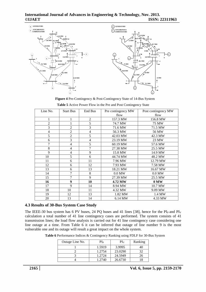
Figure 4 Pre-Contingency & Post-Contingency State of 14-Bus System


Line No. Start Bus End Bus Pre contingency MW

flow

Post contingency MW

flow

1 1 2 157.3 MW 156.8 MW

2 1 5 74.7 MW 75 MW

3 2 3 71.6 MW 71.5 MW

4 2 4 56.3 MW 56 MW

5 2 5 42.03 MW 42.3 MW

6 3 4 23.19 MW 23 MW

7 4 5 60.19 MW 57.6 MW

8 4 7 27.38 MW 25.5 MW

9 4 9 15.8 MW 14.9 MW

10 5 6 44.74 MW 48.2 MW

11 6 11 7.96 MW 12.79 MW

12 6 12 7.93 MW 7.58 MW

13 6 13 18.21 MW 16.67 MW

14 7 8 0.0 MW 0.0 MW

15 7 9 27.39 MW 25.5 MW

16 9 10 4.72 MW 0 MW

17 9 14 8.94 MW 10.7 MW

18 10 11 4.32 MW 9.09 MW

19 12 13 1.82 MW 1.4 MW

20 13 14 6.14 MW 4.33 MW


The IEEE-30 bus system has 6 PV buses, 24 PQ buses and 41 lines [38], hence for the PIP and PIV

calculation a total number of 41 line contingency cases are performed. The system consists of 41

transmission lines; the load flow analysis is carried out for 41 line contingency case considering one

line outage at a time. From Table 6 it can be inferred that outage of line number 9 is the most

vulnerable one and its outage will result a great impact on the whole system.

Table 6 Performance Indices & Contingency Ranking using FDLF for 30-Bus System

Outage Line No. PIP PIV Ranking

1 1.5919 3.9995 40

2 1.2754 23.0290 32

3 1.2724 24.5949 26

4 1.2740 26.6730 18



2166 Vol. 6, Issue 5, pp. 2159-2170

5 1.5029 23.3686 30

6 1.2978 24.1327 28

7 1.2982 23.0787 31

8 1.2692 27.3376 15

9 1.2803 29.5544 1

10 1.3611 29.1055 3

11 1.3691 26.2201 20

12 1.2786 26.3051 19

13 1.2996 18.6875 34

14 1.3727 14.5771 37

15 1.5285 9.6712 39

16 1.2967 14.2764 38

17 2.2972 0.3451 41

18 1.3477 17.2591 35

19 1.3084 24.5808 27

20 1.2928 27.9804 9

21 1.2964 27.6818 13

22 1.3078 24.8931 25

23 1.2983 27.8178 11

24 1.3005 25.2770 24

25 1.3081 20.4257 33

26 1.3000 26.1714 21

27 1.3183 24.0073 29

28 1.2953 27.0173 17

29 1.2954 28.2909 5

30 1.3109 25.7308 23

31 1.3086 27.1708 16

32 1.2960 28.3973 4

33 1.2948 29.1538 2

34 1.9801 27.6726 14

35 1.3111 26.1241 22

36 1.4453 16.6797 36

37 1.3073 27.8202 10

38 1.3211 27.7249 12

39 1.2893 28.0231 8

40 1.2964 28.1952 6

41 1.3282 28.1188 7

Figure 5 PIV Values & Contingency ranking and PIV of 30-Bus system

0 1 2 3 4 5 6 7 8 9 10 11 12 13 14 15 16 17 18 19 20 21 22 23 24 25 26 27 28 29 30 31 32 33 34 35 36 37 38 39 40 410

5

10

15

20

25

30

Outage Line Number

PIv

1 2 3 4 5 6 7 8 9 10 11 12 13 14 15 16 17 18 19 20 21 22 23 24 25 26 27 28 29 30 31 32 33 34 35 36 37 38 39 40 410

5

10

15

20

25

30

Rank of Line outage Contingency

PIv



2167 Vol. 6, Issue 5, pp. 2159-2170

Figure 5 shows the contingency ranking of this system with respect to the PIV values. Since for the

IEEE-30 bus system contingency number 9 which is the line connected between buses (6-7) is the

most critical contingency, the post contingency analysis following the outage of this line has been

done and the power flow in the post contingency state has been detailed in Figure 6. Here the system’s

bus voltages corresponding to the pre contingency and the post contingency state has been obtained,

the results are detailed in Table 7. The active power flow in all the lines during the pre-contingency

and post contingency state has been detailed in Table 8.

1

2

3

4

13

14

15

12

16

18

23

5

7

6

9

10

11

8

30

2927

28

26

25

1920

21

24

22

17

G

G

C

C

C

C

177.77 MW

83.22 MW45.71

MW

83 MW

61.9

MW

70.12 MW

14.35

MW

29.5

MW

7.89 MW

17.82 MW

7.20 MW

1.55 MW

3.65 MW

6.02 MW

2.78

MW

6.74

MW

9.02 MW

15.73 MW

7.58 MW

5.005

MW

5.64

MW

1.33

MW

3.53 MW

4.90

MW

7.09

MW3.70

MW

0.57 MW

18.81 MW

37.52

MW

Figure 6 Pre & Post contingency state of the 30-Bus System

Table 7 Bus Voltages in the Pre and Post Contingency State

Bus Number Pre-Contingency voltage

(P.U)

Post-contingency voltage (P.U)

1 1.060 1.060

2 1.043 1.043

3 1.022 1.024

4 1.013 1.016

5 1.010 1.010

6 1.012 1.015

7 1.003 0.988

8 1.010 1.010

9 1.051 1.053

10 1.044 1.047

11 1.082 1.082

12 1.057 1.059

13 1.071 1.071

14 1.042 1.044

15 1.038 1.039

16 1.045 1.046

17 1.039 1.041

18 1.028 1.030



2168 Vol. 6, Issue 5, pp. 2159-2170

19 1.025 1.027

20 1.029 1.031

21 1.032 1.034

22 1.033 1.035

23 1.027 1.029

24 1.022 1.024

25 1.019 1.021

26 1.001 1.004

27 1.026 1.028

28 1.011 1.013

29 1.006 1.009

30 0.995 0.997


Line No. Start Bus End Bus Pre contingency

MW flow

Post contingency

MW flow

1 1 2 177.77 MW 187.77 MW

2 1 3 83.22 MW 74.80 MW

3 2 4 45.71 MW 32.14 MW

4 3 4 78.01 MW 70.13 MW

5 2 5 82.99 MW 123.95 MW

6 2 6 61.91 MW 43.81 MW

7 4 6 70.12 MW 50.83 MW

8 5 7 14.35 MW 23.06 MW

9 6 7 37.52 MW 0 MW

10 6 8 29.5 MW 29.55 MW

11 6 9 27.69 MW 28.42 MW

12 6 10 15.82 MW 16.25 MW

13 9 11 0.00 MW 0.00 MW

14 9 10 27.69 MW 28.42 MW

15 4 12 44.12 MW 42.66 MW

16 12 13 0.00 MW 0.00 MW

17 12 14 7.89 MW 7.69 MW

18 12 15 17.82 MW 17.23 MW

19 12 16 7.20 MW 6.53 MW

20 14 15 1.55 MW 1.43 MW

21 16 17 3.65 MW 2.98 MW

22 15 18 6.02 MW 5.65 MW

23 18 19 2.78 MW 2.41 MW

23 19 20 6.74 MW 7.10 MW

25 10 20 9.02 MW 9.39 MW

26 10 17 5.37 MW 6.03 MW

27 10 21 15.73 MW 15.81 MW

28 10 22 7.58 MW 7.63 MW

29 21 22 1.87 MW 1.79 MW

30 15 23 5.00 MW 4.59 MW

31 22 24 5.64 MW 5.71 MW

32 23 24 1.77 MW 1.36 MW

33 24 25 1.33 MW 1.60 MW

34 25 26 3.53 MW 3.54 MW

35 25 27 4.90 MW 5.17 MW

36 28 27 18.18 MW 18.45 MW

37 27 29 6.18 MW 6.18 MW

38 27 30 7.09 MW 7.08 MW

39 29 30 3.70 MW 3.70 MW

40 8 28 0.57 MW 0.55 MW

41 6 28 18.81 MW 19.07 MW



2169 Vol. 6, Issue 5, pp. 2159-2170

V. CONCLUSIONS

In this paper, the calculation of active and reactive power performance indices for contingency

selection has been done using FDLF for various test bus systems. The post-contingency analysis

following the most severe contingency, where the bus voltages and the power flow in the entire

system has been calculated. From the results of PIP and PIV it can be concluded that for the 5-bus test

system, outage in the transmission line number 1, in IEEE 14-bus system transmission line

contingency in line number 16 and for IEEE 30-bus system, a transmission line outage in line number

9 are the most critical contingencies. An outage in these lines has the highest potential to make the

system parameters to go beyond their limits. It can be further concluded that these lines require extra

attention which can be done by providing more advanced protection schemes or load shedding

schemes.

VI. FUTURE WORK

The work discussed in this paper can be extended further by incorporating other kind of indices as

discussed in [12-13]. Calculation of the performance indices by using artificial intelligence techniques

like artificial neural networks [12] or by fuzzy logic can be taken up as future work. The contingency

analysis techniques can be further explored by considering multiple equipment failures or by

incorporating renewable energy sources in the power system.

REFERENCES

[1] Wood A.J and Wollenberg B.F., “Power generation, operation and control”, John Wiley & Sons Inc., 1996.

[2] Stott B, Alsac O and Monticelli A.J, “Security Analysis and Optimization”, Proc. IEEE, vol. 75,No. 12, pp.

1623-1644,Dec 1987.

[3] Lee C.Y and Chen N, “Distribution factors and reactive power flow in transmission line and transformer

outage studies”, IEEE Transactions on Power systems, Vol. 7,No. 1,pp. 194-200, February 1992.

[4] Singh S.N and Srivastava S.C, “Improved voltage and reactive distribution factor for outage studies”, IEEE

Transactions on Power systems, Vol. 12, No.3, pp.1085-1093, August 1997

[5] Peterson N.M, Tinney W.F and Bree D.W, “Iterative linear AC power flow solution for fast approximate

outage studies”, IEEE Transactions on Power Apparatus and Systems, Vol. PAS-91, No. 5, pp. 2048-2058,

October 1972.

[6] Brandwjn V and Lauby M.G, “Complete bounding method for A.C contingency screening”, IEEE

Transactions on Power systems, Vol. 4, No. 2, pp. 724-729, May 1989.

[7] Albuyeh F, Bose A and Heath B, “Reactive power consideration in automatic contingency selection”, IEEE

Transactions on Power systems, Vol. PAS-101, No. 1, pp. 107-112, January 1982.

[8] Zaborzky J, Whang K.W and Prasad K, “Fast contingency evaluation using concentric relaxation”, IEEE

Transactions on Power systems, Vol. PAS-99, No. 1, pp. 28-36, February 1980.

[9] Stott B and Alsac O, “Fast decoupled load flow”, IEEE Transactions on Power Apparatus and Systems, Vol.

PAS-91, No. 5, pp. 859-869, May 1974.

[10] Ejebe G.C and Wollenberg B.F, “Automatic Contingency Selection”, IEEE Transactions on Power

Apparatus and Systems, Vol. PAS-98, No. 1, pp. 97-109, January 1979.

[11] Innocent Kamwa, Robert Grondin and Lester Loud, “Time- Varying Contingency Screening for Dynamic

Security Assessment Using Intelligent-Systems Techniques”, IEEE Transactions on Power Systems, Vol. 16,

No. 3, pp. 526-537, August 2001

[12] T.Jain, L.Srivastava, S.N. Singh and Arvind Jain, “Parallel Radial Basis Function Neural Network Based

Fast Voltage Estimation for Contingency Analysis”, IEEE International Conference on Electric Utility

Deregulation, Restructuring and Power Technologies, Hong Kong, April 2004.

[13] F. Fatehi, M.Rashidinejad and A.A Gharaveisi, “Contingency Ranking Based on a Voltage Stability

Criteria Index”, IEEE Transactions in Power System, 2007

[14] Vaibhav Donde, Vanessa Lopex, Bernard Lesieutre, Ali Pinar, Chao Yang and Juan Meza, “Severe

Multiple Contingency Screening in Electric Power Systems”, IEEE Transactions on Power Systems, Vol.23,

No.2, pp. 406-417, May 2008.

[15] Magnus Perninge, Flip Linskog and Lennart Soder, “Importance Sampling of Injected Powers for Electric

Power System Security Analysis”, IEEE Transactions on Power Systems, Vol.27, No.1, February 2012.



2170 Vol. 6, Issue 5, pp. 2159-2170

AUTHORS BIOGRAPHIES

Amit Kumar Roy was born in West Bengal, India on February, 1988. He received his B.E

degree in Electrical & Electronics Engineering from Sathyabama University, Chennai in

2009 and M.E degree in Power Systems & Electric drives from Thapar University, Patiala

in 2011. He had secured Gold Medal in his M.E degree and 2nd position in his B.E degree.

He is also a life member of Indian Society of Technical Education (ISTE), New Delhi. At

present he is working as an Assistant Professor in the Department of Electrical Engineering

at JSS Academy of Technical Education, Noida, U.P. where he is actively involved in the

academic activities and research work. His area of interest includes intelligent techniques applications to Power

Systems, Power Converters and Electric Drives.

Sanjay Kr. Jain was born in Madhya Pradesh, India on December, 1971. Awarded B.E.

(Electrical Engineering) from SGSITS Indore in 1992. Awarded M.E. (Power System) from

University of Roorkee (UOR), Roorkee in 1995. Awarded Ph.D. from IIT Roorkee in 2001.

Dr. Jain has a vast teaching experience of 13 years since 2001. At present he is working as

an Associate Professor in the Department of Electrical & Instrumentation Engineering at

Thapar University, Patiala, Punjab. His main area of interest lies in various techniques in

Powers System Optimization and modeling of Self Excited Induction Generators.

improved t line contingency analysis in power … · system is essential for contingency analysis...

Documents