intermediary leverage cycles and financial stability/media/others/events/2013/bank... ·...
TRANSCRIPT
Intermediary Leverage Cycles and Financial Stability Tobias Adrian and Nina Boyarchenko The views presented here are the authors’ and are not representative of the views of the Federal Reserve Bank of New York or of the Federal Reserve System
Introduction
Questions about Financial Stability Policy
Systemic distress of financial intermediaries raises questions aboutfinancial stability policies:
How does capital regulation affect the trade-off between the pricing ofcredit and the amount of systemic risk?
How does macroprudential policy function in equilibrium?
What are the welfare implications of capital regulation?
We develop a theoretical framework to address these questions
T. Adrian, N. Boyarchenko Intermediary Leverage Cycles May 8, 2013 2
Introduction
Our Approach
We use a standard macro model with a financial sector and add onekey assumption:
Funding constraints of financial intermediaries are risk based, sointermediaries have to hold more capital when the riskiness of theirassets increases
This assumption is empirically motivated from risk managementpractices and regulatory constraints
Equilibrium dynamics capture stylized facts:
Procyclical leverage of intermediary balance sheetsProcyclical share of intermediated creditRelationship between asset risk premia and intermediary leverage
T. Adrian, N. Boyarchenko Intermediary Leverage Cycles May 8, 2013 3

The Model
Economy Structure
Producersrandom dividendstream, At, per unitof project financed bydirect borrowing fromintermediaries andhouseholds
Intermediariesfinanced by house-holds against capitalinvestments
Householdssolve portfolio choiceproblem betweenholding intermedi-ary debt, physicalcapital and risk-freeborrowing/lending
Atkht
it
Atkt
Cbtbht
1
T. Adrian, N. Boyarchenko Intermediary Leverage Cycles May 8, 2013 4
The Model
Production
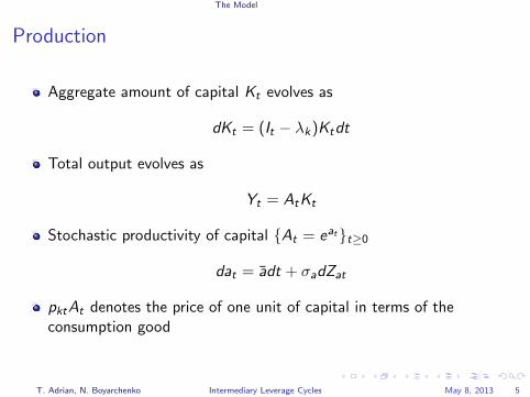
Aggregate amount of capital Kt evolves as
dKt = (It − λk)Ktdt
Total output evolves as
Yt = AtKt
Stochastic productivity of capital {At = eat}t≥0
dat = adt + σadZat
pktAt denotes the price of one unit of capital in terms of theconsumption good
T. Adrian, N. Boyarchenko Intermediary Leverage Cycles May 8, 2013 5
The Model
Households
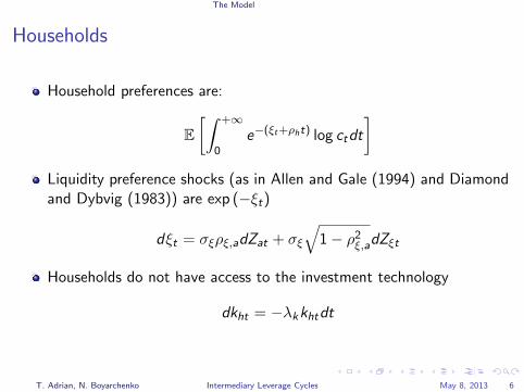
Household preferences are:
E[∫ +∞
0e−(ξt+ρht) log ctdt
]Liquidity preference shocks (as in Allen and Gale (1994) and Diamondand Dybvig (1983)) are exp (−ξt)
dξt = σξρξ,adZat + σξ
√1− ρ2
ξ,adZξt
Households do not have access to the investment technology
dkht = −λkkhtdt
T. Adrian, N. Boyarchenko Intermediary Leverage Cycles May 8, 2013 6
The Model
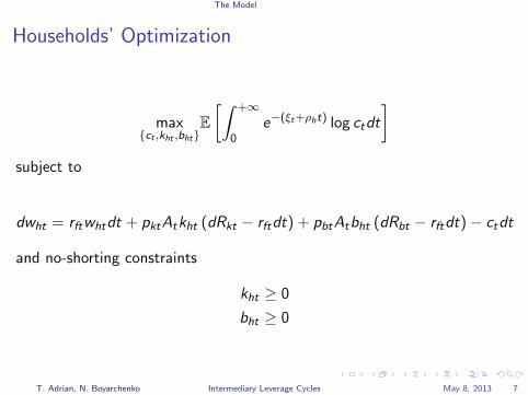
Households’ Optimization
max{ct ,kht ,bht}
E[∫ +∞
0e−(ξt+ρht) log ctdt
]subject to
dwht = rftwhtdt + pktAtkht (dRkt − rftdt) + pbtAtbht (dRbt − rftdt)− ctdt
and no-shorting constraints
kht ≥ 0
bht ≥ 0
T. Adrian, N. Boyarchenko Intermediary Leverage Cycles May 8, 2013 7

The Model
Intermediaries
Financial intermediaries create new capital
dkt = (Φ(it)− λk) ktdt
Investment carries quadratic adjustment costs (Brunnermeier andSannikov (2012))
Φ (it) = φ0
(√1 + φ1it − 1
)Intermediaries finance investment projects through inside equity andoutside risky debt giving the budget constraint
pktAtkt = pbtAtbt + wt
T. Adrian, N. Boyarchenko Intermediary Leverage Cycles May 8, 2013 8

The Model
Intermediaries’ Risk Based Capital Constraint
Risk based capital constraint (Danielsson, Shin, and Zigrand (2011))
α
√1
dt〈ktd (pktAt)〉2 = wt
Implies a time-varying leverage constraint
θt =pktAtkt
wt=
1
α
√1dt
⟨d(pktAt)pktAt
⟩2
Note that the constraint is such that intermediary equity isproportional to the Value-at-Risk of total assets
This will imply that default probabilities vary over time
Microfoundation of the risk based capital constraint is provided inAdrian and Shin (2010)
T. Adrian, N. Boyarchenko Intermediary Leverage Cycles May 8, 2013 9

The Model
Risk-based Capital Constraints
VaR is the potential loss in value of inventory positions due toadverse market movements over a defined time horizon with aspecified confidence level. We typically employ a one-day timehorizon with a 95% confidence level.
Source: Goldman Sachs 2011 Annual Report
More
T. Adrian, N. Boyarchenko Intermediary Leverage Cycles May 8, 2013 10
The Model
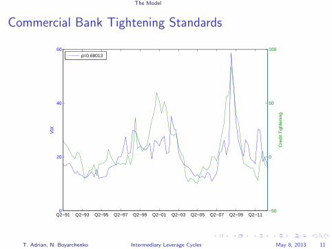
Commercial Bank Tightening Standards
Q2−91 Q2−93 Q2−95 Q2−97 Q2−99 Q2−01 Q2−03 Q2−05 Q2−07 Q2−09 Q2−110
20
40
60V
IX
−50
0
50
100
Cre
dit T
ight
enin
g
ρ=0.68013
T. Adrian, N. Boyarchenko Intermediary Leverage Cycles May 8, 2013 11
The Model
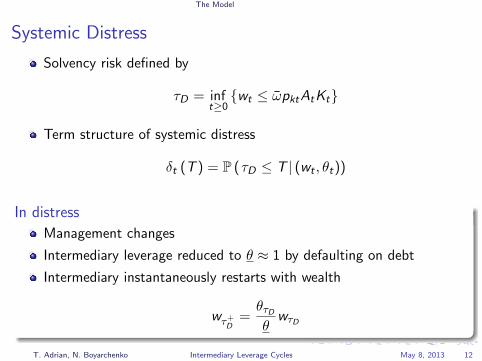
Systemic Distress
Solvency risk defined by
τD = inft≥0{wt ≤ ωpktAtKt}
Term structure of systemic distress
δt (T ) = P (τD ≤ T | (wt , θt))
In distress
Management changes
Intermediary leverage reduced to θ ≈ 1 by defaulting on debt
Intermediary instantaneously restarts with wealth
wτ+D
=θτDθ
wτD
T. Adrian, N. Boyarchenko Intermediary Leverage Cycles May 8, 2013 12

The Model
Intermediaries’ Optimization
Intermediary maximizes equity holder value to solve
max{kt ,βt ,it}
E[∫ τD
0e−ρtwtdt
]subject to the dynamic intermediary budget constraint
dwt = ktpktAt (dRkt + (Φ (it)− it/pkt) dt)− btpbtAtdRbt
and the risk based capital constraint
α
√1
dt〈ktd (pktAt)〉2 = wt
T. Adrian, N. Boyarchenko Intermediary Leverage Cycles May 8, 2013 13
The Model
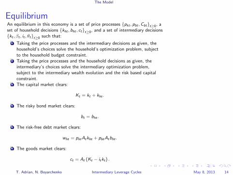
EquilibriumAn equilibrium in this economy is a set of price processes {pkt , pbt ,Cbt}t≥0, aset of household decisions {kht , bht , ct}t≥0, and a set of intermediary decisions{kt , βt , it , θt}t≥0 such that:
1 Taking the price processes and the intermediary decisions as given, thehousehold’s choices solve the household’s optimization problem, subjectto the household budget constraint.
2 Taking the price processes and the household decisions as given, theintermediary’s choices solve the intermediary optimization problem,subject to the intermediary wealth evolution and the risk based capitalconstraint.
3 The capital market clears:
Kt = kt + kht .
4 The risky bond market clears:
bt = bht .
5 The risk-free debt market clears:
wht = pktAtkht + pbtAtbht .
6 The goods market clears:
ct = At (Kt − itkt) .
T. Adrian, N. Boyarchenko Intermediary Leverage Cycles May 8, 2013 14

The Model
Related Literature
Leverage Cycles: Geanakoplos (2003), Fostel and Geanakoplos(2008), Brunnermeier and Pedersen (2009)
Amplification in Macroeconomy: Bernanke and Gertler (1989),Kiyotaki and Moore (1997)
Financial Intermediaries and the Macroeconomy: Gertler andKiyotaki (2012), Gertler, Kiyotaki, and Queralto (2011), He andKrishnamurthy (2012, 2013), Brunnermeier and Sannikov (2011,2012)
T. Adrian, N. Boyarchenko Intermediary Leverage Cycles May 8, 2013 15
Solution
Solution Strategy
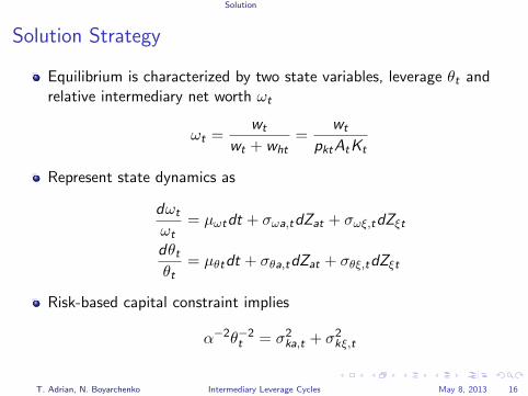
Equilibrium is characterized by two state variables, leverage θt andrelative intermediary net worth ωt
ωt =wt
wt + wht=
wt
pktAtKt
Represent state dynamics as
dωt
ωt= µωtdt + σωa,tdZat + σωξ,tdZξt
dθtθt
= µθtdt + σθa,tdZat + σθξ,tdZξt
Risk-based capital constraint implies
α−2θ−2t = σ2
ka,t + σ2kξ,t
T. Adrian, N. Boyarchenko Intermediary Leverage Cycles May 8, 2013 16

Solution
Volatility Risk
−5 0 5−4
−2
0
2
4
Lagged Volatility Growth
Leve
rage
Gro
wth
−0.5 0 0.5 1−1
−0.5
0
0.5
1
Lagged VIX Growth
Leve
rage
Gro
wth
y = 0.00074 − 0.12xR2 = 0.013
y = 0.014 − 0.21xR2 = 0.053
Data Mean 5% Median 95%
β0 0.014 0.000 -0.003 0.000 0.003β1 -0.208 -0.105 -0.187 -0.104 -0.025R2 0.053 0.013 0.001 0.011 0.035
Simulation details
T. Adrian, N. Boyarchenko Intermediary Leverage Cycles May 8, 2013 17
Solution
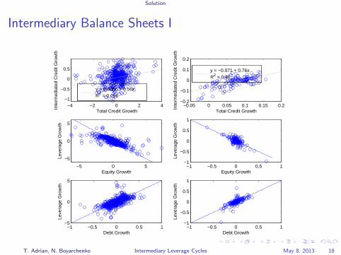
Intermediary Balance Sheets I
−4 −2 0 2 4−1
−0.5
0
0.5
Total Credit Growth
Inte
rmed
iate
d C
redi
t Gro
wth
−5 0 5
−5
0
5
Equity Growth
Leve
rage
Gro
wth
−1 −0.5 0 0.5 1−5
0
5
Debt Growth
Leve
rage
Gro
wth
−0.05 0 0.05 0.1 0.15 0.2−0.2
−0.1
0
0.1
0.2
Total Credit Growth
Inte
rmed
iate
d C
redi
t Gro
wth
−1 −0.5 0 0.5 1−1
−0.5
0
0.5
1
Equity GrowthLe
vera
ge G
row
th
−1 −0.5 0 0.5 1−1
−0.5
0
0.5
1
Debt Growth
Leve
rage
Gro
wth
y = 0.0086 + 0.56xR2 = 0.056
y = −0.071 + 0.76xR2 = 0.46
T. Adrian, N. Boyarchenko Intermediary Leverage Cycles May 8, 2013 18
Solution
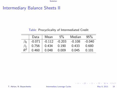
Intermediary Balance Sheets II
Table: Procyclicality of Intermediated Credit
Data Mean 5% Median 95%
β0 -0.071 -0.112 -0.203 -0.108 -0.040β1 0.756 0.434 0.190 0.433 0.680R2 0.460 0.048 0.009 0.045 0.101
T. Adrian, N. Boyarchenko Intermediary Leverage Cycles May 8, 2013 19
Solution
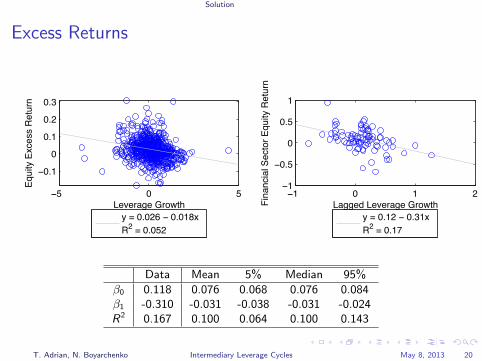
Excess Returns
−5 0 5
−0.1
0
0.1
0.2
0.3
Leverage Growth
Equi
ty E
xces
s R
etur
n
−1 0 1 2−1
−0.5
0
0.5
1
Lagged Leverage GrowthFina
ncia
l Sec
tor E
quity
Ret
urn
y = 0.026 − 0.018xR2 = 0.052
y = 0.12 − 0.31xR2 = 0.17
Data Mean 5% Median 95%
β0 0.118 0.076 0.068 0.076 0.084β1 -0.310 -0.031 -0.038 -0.031 -0.024R2 0.167 0.100 0.064 0.100 0.143
T. Adrian, N. Boyarchenko Intermediary Leverage Cycles May 8, 2013 20
Solution
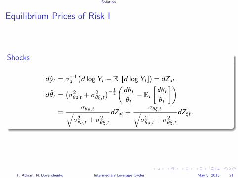
Equilibrium Prices of Risk I
Shocks
dyt = σ−1a (d log Yt − Et [d log Yt ]) = dZat
d θt =(σ2θa,t + σ2
θξ,t
)− 12
(dθtθt− Et
[dθtθt
])=
σθa,t√σ2θa,t + σ2
θξ,t
dZat +σθξ,t√
σ2θa,t + σ2
θξ,t
dZξt .
T. Adrian, N. Boyarchenko Intermediary Leverage Cycles May 8, 2013 21
Solution
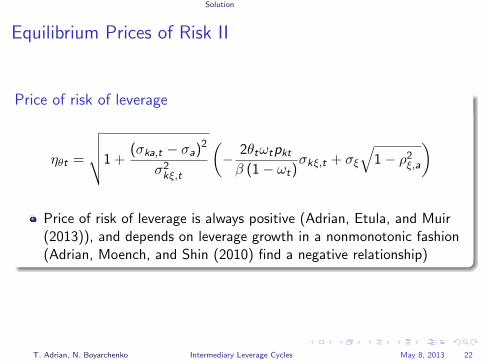
Equilibrium Prices of Risk II
Price of risk of leverage
ηθt =
√√√√1 +(σka,t − σa)2
σ2kξ,t
(− 2θtωtpkt
β (1− ωt)σkξ,t + σξ
√1− ρ2
ξ,a
)
Price of risk of leverage is always positive (Adrian, Etula, and Muir(2013)), and depends on leverage growth in a nonmonotonic fashion(Adrian, Moench, and Shin (2010) find a negative relationship)
T. Adrian, N. Boyarchenko Intermediary Leverage Cycles May 8, 2013 22

Solution
Equilibrium Prices of Risk III
−4 −2 0 2 4 6 8 10 12 14−4
−2
0
2
4
6
8
10
12
14
S1B1
S1B2 S1B3
S1B4
S1B5
S2B1
S2B2
S2B3 S2B4
S2B5
S3B1
S3B2 S3B3
S3B4
S3B5
S4B1 S4B2
S4B3
S4B4 S4B5
S5B1
S5B2 S5B3
S5B4
S5B5
Mom 1
Mom 2
Mom 3Mom 4Mom 5
Mom 6Mom 7
Mom 8Mom 9
Mom10
0−1yr
5−10y1−2yr
2−3yr3−4yr4−5yr
Predicted Expected Return
Rea
lized
Mea
n R
etur
n
Figure: Source: Adrian, Etula, and Muir (2013)
T. Adrian, N. Boyarchenko Intermediary Leverage Cycles May 8, 2013 23

Solution
Equilibrium Prices of Risk IV
Price of risk of output
ηyt = σa + σξ
(ρξ,a −
σka,t − σaσkξ,t
√1− ρ2
ξ,a
)
Switches sign, consistent with insignificant estimates of price ofoutput risk
Usually becomes negative when exposure to liquidity shock is small
T. Adrian, N. Boyarchenko Intermediary Leverage Cycles May 8, 2013 24

Distortions and Amplification
Term Structure of Systemic Risk
0 0.5 1 1.5 2 2.5 3 3.5 4 4.5 50
0.1
0.2
0.3
0.4
0.5
0.6
0.7
0.8
0.9
1
Horizon
Dis
tres
s pr
obab
ility
α=2α=4
T. Adrian, N. Boyarchenko Intermediary Leverage Cycles May 8, 2013 25
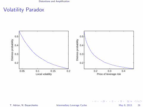
Distortions and Amplification
Volatility Paradox
0.05 0.1 0.15 0.2
0.2
0.3
0.4
0.5
Local volatility
Dis
tres
s pr
obab
ility
0.2 0.3 0.4
0.2
0.3
0.4
0.5
Price of leverage riskD
istr
ess
prob
abili
ty
T. Adrian, N. Boyarchenko Intermediary Leverage Cycles May 8, 2013 26
Distortions and Amplification
Constant Leverage Benchmark
Constant expected output and consumption growth
But lower level of output and consumption growth
Constant investment and price of capital
Liquidity shocks have no impact on real activity
T. Adrian, N. Boyarchenko Intermediary Leverage Cycles May 8, 2013 27

Distortions and Amplification
A Sample Path of the Economy
0 10 20 30 40 50 60 704
6
8
Year
Out
put
0 10 20 30 40 50 60 704
6
8
Cons
umpt
ion
0 10 20 30 40 50 60 70
0.20.40.60.8
Year
Wea
lth
0 10 20 30 40 50 60 70
5101520
Year
Leve
rage
0 10 20 30 40 50 60 70−0.2−0.1
00.1
Year
Equi
ty R
etur
n
T. Adrian, N. Boyarchenko Intermediary Leverage Cycles May 8, 2013 28

Distortions and Amplification
Household Welfare
2 4 6 8 10α
Wel
fare
2 4 6 8 10
0.2
0.4
0.6
0.8
1
αD
istr
ess
prob
abili
ty
6 month1 year5 year
T. Adrian, N. Boyarchenko Intermediary Leverage Cycles May 8, 2013 29
Distortions and Amplification
Conclusion
Dynamic, general equilibrium theory of financial intermediaries’leverage cycle with endogenous amplification and endogenoussystemic risk
Conceptual basis for policies towards financial stability
Systemic risk return trade-off: tighter intermediary capitalrequirements tend to shift the term structure of systemic downward,at the cost of increased prices of risk today
Model captures important stylized facts:1 Procyclical intermediary leverage2 Procyclicality of intermediated credit3 Financial sector equity return and intermediary leverage growth4 Exposure to intermediary leverage shocks as pricing factor
T. Adrian, N. Boyarchenko Intermediary Leverage Cycles May 8, 2013 30
Distortions and Amplification
Tobias Adrian and Hyun Song Shin. Procyclical Leverage and Value-at-Risk.Federal Reserve Bank of New York Staff Reports No. 338, 2010.
Tobias Adrian, Emanuel Moench, and Hyun Song Shin. Financial Intermediation,Asset Prices, and Macroeconomic Dynamics. Federal Reserve Bank of NewYork Staff Reports No. 442, 2010.
Tobias Adrian, Erkko Etula, and Tyler Muir. Financial Intermediaries and theCross-Section of Asset Returns. Journal of Finance, 2013. Forthcoming.
Franklin Allen and Douglas Gale. Limited market participation and volatility ofasset prices. American Economic Review, 84:933–955, 1994.
Ben Bernanke and Mark Gertler. Agency Costs, Net Worth, and BusinessFluctuations. American Economic Review, 79(1):14–31, 1989.
Markus K. Brunnermeier and Lasse Heje Pedersen. Market Liquidity and FundingLiquidity. Review of Financial Studies, 22(6):2201–2238, 2009.
Markus K. Brunnermeier and Yuliy Sannikov. The I Theory of Money.Unpublished working paper, Princeton University, 2011.
Markus K. Brunnermeier and Yuliy Sannikov. A Macroeconomic Model with aFinancial Sector. Unpublished working paper, Princeton University, 2012.
T. Adrian, N. Boyarchenko Intermediary Leverage Cycles May 8, 2013 31
Distortions and Amplification
Jon Danielsson, Hyun Song Shin, and Jean-Pierre Zigrand. Balance sheetcapacity and endogenous risk. Working Paper, 2011.
Douglas W. Diamond and Philip H. Dybvig. Bank runs, deposit insurance andliquidity. Journal of Political Economy, 93(1):401–419, 1983.
Ana Fostel and John Geanakoplos. Leverage Cycles and the Anxious Economy.American Economic Review, 98(4):1211–1244, 2008.
John Geanakoplos. Liquidity, Default, and Crashes: Endogenous Contracts inGeneral Equilibrium. In M. Dewatripont, L.P. Hansen, and S.J. Turnovsky,editors, Advances in Economics and Econometrics II, pages 107–205.Econometric Society, 2003.
Mark Gertler and Nobuhiro Kiyotaki. Banking, Liquidity, and Bank Runs in anInfinite Horizon Economy. Unpublished working papers, Princeton University,2012.
Mark Gertler, Nobuhiro Kiyotaki, and Albert Queralto. Financial Crises, BankRisk Exposure, and Government Financial Policy. Unpublished working papers,Princeton University, 2011.
Zhiguo He and Arvind Krishnamurthy. A Model of Capital and Crises. Review ofEconomic Studies, 79(2):735–777, 2012.
T. Adrian, N. Boyarchenko Intermediary Leverage Cycles May 8, 2013 32
Distortions and Amplification
Zhiguo He and Arvind Krishnamurthy. Intermediary Asset Pricing. AmericanEconomic Review, 103(2):732–770, 2013.
Nobuhiro Kiyotaki and John Moore. Credit Cycles. Journal of Political Economy,105(2):211–248, 1997.
T. Adrian, N. Boyarchenko Intermediary Leverage Cycles May 8, 2013 33

Empirical Evidence
Broker-Dealer Balance Sheets: Levels
5
7
9
11
13
15
17
19
21
23
25
0
0.5
1
1.5
2
2.5
3
3.5
2000 2002 2004 2006 2008 2010 2012
Dollars (trillions)
Source: Flow of Funds
Total Assets(left axis)
Total Liabilities(left axis)
Leverage(right axis)
Security Broker-Dealer: Assets, Liabilies, Equity, LeverageAssets to Equity
Back
T. Adrian, N. Boyarchenko Intermediary Leverage Cycles May 8, 2013 34

Empirical Evidence
Broker-Dealer Balance Sheets: Annual Growth
-50
-40
-30
-20
-10
0
10
20
30
40
-50
-40
-30
-20
-10
0
10
20
30
40
2000 2002 2004 2006 2008 2010 2012
Percent
Source: Flow of Funds
Percent
Equity
Total Assets
Total Liabilities
Leverage
Security Broker-Dealer: Assets, Liabilies, Equity, Leverage
Back
T. Adrian, N. Boyarchenko Intermediary Leverage Cycles May 8, 2013 35

Empirical Evidence
Broker-Dealer Balance Sheets: Adjustments
-1500
-1000
-500
0
500
1000
-1500 -1000 -500 0 500 1000
Security Broker Dealer Change of Assets as a Function of Change in Equity and in Liabilities (Annual)
Liabilities Changes
Equity Changes
Source: Federal Reserve Flow of Funds. Equity is at book value. -0.2
-0.1
0
0.1
0.2
0.3
0.4
0.5
0.6
Jan-95 Jan-97 Jan-99 Jan-01 Jan-03 Jan-05 Jan-07 Jan-09
Equity Growth
Issuance Growth
Back
T. Adrian, N. Boyarchenko Intermediary Leverage Cycles May 8, 2013 36
Empirical Evidence
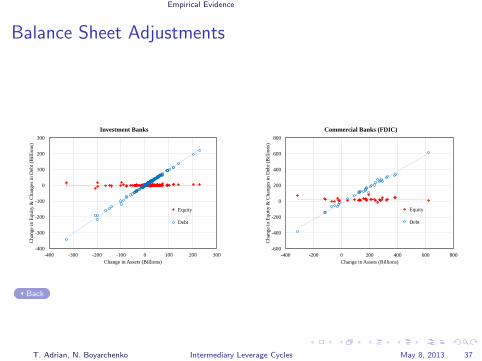
Balance Sheet Adjustments
-400
-300
-200
-100
0
100
200
300
-400 -300 -200 -100 0 100 200 300
Cha
nge
in E
quity
& C
hang
es in
Deb
t (B
illio
ns)
Change in Assets (Billions)
Investment Banks
Equity
Debt
-600
-400
-200
0
200
400
600
800
-400 -200 0 200 400 600 800
Cha
nge
in E
quity
& C
hang
es in
Deb
t (B
illio
ns)
Change in Assets (Billions)
Commercial Banks (FDIC)
Equity
Debt
Back
T. Adrian, N. Boyarchenko Intermediary Leverage Cycles May 8, 2013 37
Empirical Evidence
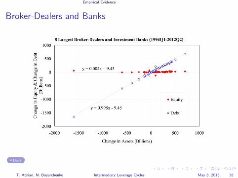
Broker-Dealers and Banks
Back
T. Adrian, N. Boyarchenko Intermediary Leverage Cycles May 8, 2013 38

Empirical Evidence
Broker-Dealer VaR
T. Adrian, N. Boyarchenko Intermediary Leverage Cycles May 8, 2013 39
Empirical Evidence
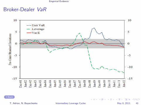
Broker-Dealer VaR
Back
T. Adrian, N. Boyarchenko Intermediary Leverage Cycles May 8, 2013 40

Additional Results
Simulation Parameters
Parameter Value
a 0.0651σa 0.388ρ 0.06
ρh − σ2ξ/2 0.05
φ0 0.1φ1 20λk 0.03
ρξ,a 0σξ 0.0388α 2.5
Ref.: Brunnermeier and Sannikov (2012)
Monthly simulation frequency
10000 paths; 70 years Back
T. Adrian, N. Boyarchenko Intermediary Leverage Cycles May 8, 2013 41
Additional Results
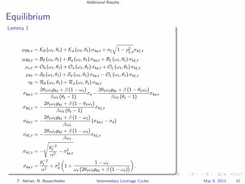
EquilibriumLemma 1
µRk,t = K0 (ωt , θt) +Ka (ωt , θt)σka,t + σξ
√1− ρ2
ξ,aσkξ,t
µRb,t = B0 (ωt , θt) + Ba (ωt , θt)σka,t + Bξ (ωt , θt)σkξ,t
µωt = O0 (ωt , θt) +Oa (ωt , θt)σka,t +Oξ (ωt , θt)σkξ,t
µθt = S0 (ωt , θt) + Sa (ωt , θt)σka,t −Oξ (ωt , θt)σkξ,t
rft = R0 (ωt , θt) +Ra (ωt , θt)σka,t
σba,t =2θtωtpkt + β (1− ωt)
βωt (θt − 1)σa −
2θtωtpkt + β (1− θtωt)
βωt (θt − 1)σka,t
σbξ,t = −2θtωtpkt + β (1− θtωt)
βωt (θt − 1)σkξ,t
σθa,t = −2θtωtpkt + β (1− ωt)
βωt(σka,t − σa)
σθξ,t = −2θtωtpkt + β (1− ωt)
βωtσkξ,t
σkξ,t = −
√θ−2t
α2− σ2
ka,t
σka,t =θ−2t
α2+ σ2
a
(1 +
1− ωt
ωt (2θtωtpkt + β (1− ωt))
).
T. Adrian, N. Boyarchenko Intermediary Leverage Cycles May 8, 2013 42
Additional Results
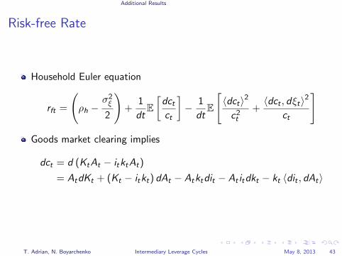
Risk-free Rate
Household Euler equation
rft =
(ρh −
σ2ξ
2
)+
1
dtE[
dctct
]− 1
dtE
[〈dct〉2
c2t
+〈dct , dξt〉2
ct
]
Goods market clearing implies
dct = d (KtAt − itktAt)
= AtdKt + (Kt − itkt) dAt − Atktdit − At itdkt − kt 〈dit , dAt〉
T. Adrian, N. Boyarchenko Intermediary Leverage Cycles May 8, 2013 43
Additional Results
Stress Tests
Inherent limitations to VaR include [. . . ] VaR does not estimatepotential losses over longer time horizons where moves may beextreme.
T. Adrian, N. Boyarchenko Intermediary Leverage Cycles May 8, 2013 44
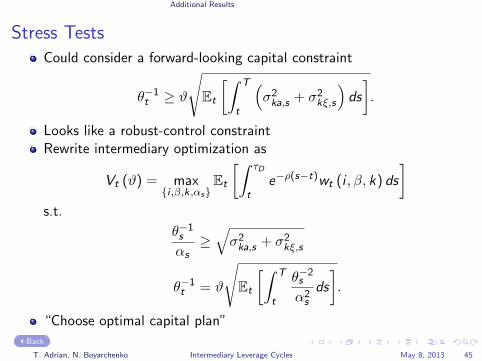
Additional Results
Stress TestsCould consider a forward-looking capital constraint
θ−1t ≥ ϑ
√Et
[∫ T
t
(σ2ka,s + σ2
kξ,s
)ds
].
Looks like a robust-control constraintRewrite intermediary optimization as
Vt (ϑ) = max{i ,β,k,αs}
Et
[∫ τD
te−ρ(s−t)wt (i , β, k) ds
]s.t.
θ−1s
αs≥√σ2ka,s + σ2
kξ,s
θ−1t = ϑ
√Et
[∫ T
t
θ−2s
α2s
ds
].
“Choose optimal capital plan”
Back
T. Adrian, N. Boyarchenko Intermediary Leverage Cycles May 8, 2013 45

Extensions
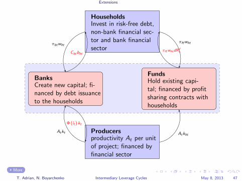
Alternative Specification
Two financial sectors: banks and funds
Leveraged intermediaries have VaR constraint (as in the currentpaper) while funds have skin in the game constraint (as in He andKrishnamurthy (2012, 2013))
Bank managers, fund managers, and households have log utility
VaR constraint sometimes binds
T. Adrian, N. Boyarchenko Intermediary Leverage Cycles May 8, 2013 46
Extensions
HouseholdsInvest in risk-free debt,non-bank financial sec-tor and bank financialsector
BanksCreate new capital; fi-nanced by debt issuanceto the households
FundsHold existing capi-tal; financed by profitsharing contracts withhouseholds
Producersproductivity At per unitof project; financed byfinancial sector
πbtwhtπftwht
CbtbhtπftwhtdR f
t
Atkt Atkht
Φ (it) kt
More
T. Adrian, N. Boyarchenko Intermediary Leverage Cycles May 8, 2013 47
Extensions
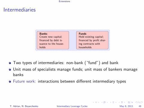
Intermediaries
BanksCreate new capital;financed by debt is-suance to the house-holds
FundsHold existing capital;financed by profit shar-ing contracts withhouseholds
Two types of intermediaries: non-bank (“fund”) and bank
Unit mass of specialists manage funds; unit mass of bankers managebanks
Future work: interactions between different intermediary types
T. Adrian, N. Boyarchenko Intermediary Leverage Cycles May 8, 2013 48
Extensions
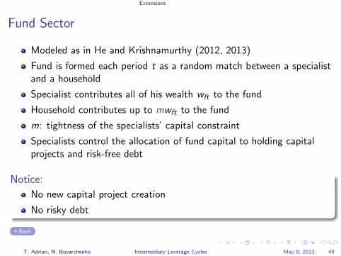
Fund Sector
Modeled as in He and Krishnamurthy (2012, 2013)
Fund is formed each period t as a random match between a specialistand a household
Specialist contributes all of his wealth wft to the fund
Household contributes up to mwft to the fund
m: tightness of the specialists’ capital constraint
Specialists control the allocation of fund capital to holding capitalprojects and risk-free debt
Notice:
No new capital project creation
No risky debt
Back
T. Adrian, N. Boyarchenko Intermediary Leverage Cycles May 8, 2013 49
Extensions
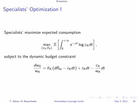
Specialists’ Optimization I
Specialists’ maximize expected consumption
max{cft ,θft}
E[∫ +∞
0e−ρt log cftdt
],
subject to the dynamic budget constraint
dwft
wft= θft (dRkt − rftdt) + rftdt − cft
wftdt
T. Adrian, N. Boyarchenko Intermediary Leverage Cycles May 8, 2013 50

Extensions
Specialists’ Optimization II
Lemma 2
The specialists consume a constant fraction of their wealth
cft = ρwft ,
and allocate the fund’s capital as a mean-variance investor
θft =µRk,t − rftσ2ka,t + σ2
kξ,t
.
Back
T. Adrian, N. Boyarchenko Intermediary Leverage Cycles May 8, 2013 51
Extensions
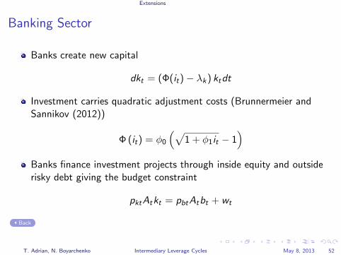
Banking Sector
Banks create new capital
dkt = (Φ(it)− λk) ktdt
Investment carries quadratic adjustment costs (Brunnermeier andSannikov (2012))
Φ (it) = φ0
(√1 + φ1it − 1
)Banks finance investment projects through inside equity and outsiderisky debt giving the budget constraint
pktAtkt = pbtAtbt + wt
Back
T. Adrian, N. Boyarchenko Intermediary Leverage Cycles May 8, 2013 52
Extensions
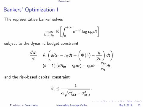
Bankers’ Optimization I
The representative banker solves
maxθt ,it ,cbt
E[∫ +∞
0e−ρt log cbtdt
]subject to the dynamic budget constraint
dwt
wt= θt
(dRkt − rftdt +
(Φ (it)−
itpkt
)dt
)− (θ − 1) (dRbt − rftdt) + rftdt − cbt
wtdt,
and the risk-based capital constraint
θt ≤1
α√σ2ka,t + σ2
kξ,t
.
T. Adrian, N. Boyarchenko Intermediary Leverage Cycles May 8, 2013 53
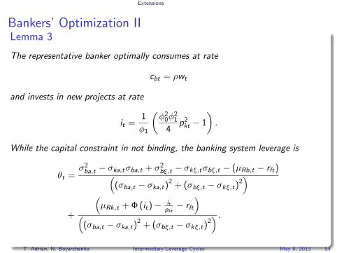
Extensions
Bankers’ Optimization IILemma 3
The representative banker optimally consumes at rate
cbt = ρwt
and invests in new projects at rate
it =1
φ1
(φ2
0φ21
4p2kt − 1
).
While the capital constraint in not binding, the banking system leverage is
θt =σ2ba,t − σka,tσba,t + σ2
bξ,t − σkξ,tσbξ,t − (µRb,t − rft)((σba,t − σka,t)2 + (σbξ,t − σkξ,t)2
)+
(µRk,t + Φ (it)− it
pkt− rft
)(
(σba,t − σka,t)2 + (σbξ,t − σkξ,t)2) .
Back
T. Adrian, N. Boyarchenko Intermediary Leverage Cycles May 8, 2013 54
Extensions
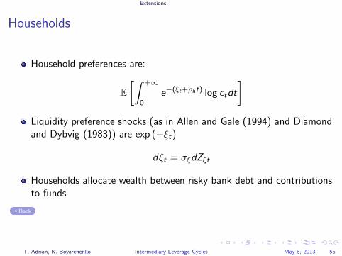
Households
Household preferences are:
E[∫ +∞
0e−(ξt+ρht) log ctdt
]Liquidity preference shocks (as in Allen and Gale (1994) and Diamondand Dybvig (1983)) are exp (−ξt)
dξt = σξdZξt
Households allocate wealth between risky bank debt and contributionsto funds
Back
T. Adrian, N. Boyarchenko Intermediary Leverage Cycles May 8, 2013 55

Extensions
Households’ Optimization IThe representative household solves
maxπkt ,πbt
ct
E[∫ +∞
0e−ξt−ρht log ctdt
],
subject to the dynamic budget constraint
dwht
wht= πktθft (dRkt − rftdt) + πbt (dRbt − rftdt) + rftdt − ct
whtdt,
the skin-in-the-game constraint
πktwht ≤ mwft ,
and no shorting constraints
πkt ≥ 0
bht ≥ 0.
T. Adrian, N. Boyarchenko Intermediary Leverage Cycles May 8, 2013 56

Extensions
Households’ Optimization II
Lemma 4
The households’ optimal consumption choice satisfies
ct =
(ρh −
σ2ξ
2
)wht .
While the households are unconstrained in their wealth allocation, the households’optimal portfolio choice is given by[
πktπbt
]=
([θftσka,t θftσkξ,tσba,t σbξ,t
] [θftσka,t σba,tθftσkξ,t σbξ,t
])−1 [θft (µRk,t − rft)µRb,t − rft
]−[θftσka,t σba,tθftσkξ,t σbξ,t
]−1 [0σξ
].
Back
T. Adrian, N. Boyarchenko Intermediary Leverage Cycles May 8, 2013 57

Extensions
EquilibriumAn equilibrium in the economy is a set of price processes {pkt , pbt , rft}t≥0, aset of household decisions {πkt , bht , ct}t≥0, a set of specialist decisions{kft , cft}t≥0, and a set of intermediary decisions {kt , it , bt , cbt}t≥0 such thatthe following apply:
1 Taking the price processes, the specialist decisions and the intermediarydecisions as given, the household’s choices solve the household’soptimization problem, subject to the household budget constraint, the noshorting constraints and the skin-in-the-game constraint for the funds.
2 Taking the price processes, the specialist decisions and the householddecisions as given, the intermediary’s choices solve the intermediary’soptimization problem, subject to the intermediary budget constraint, andthe regulatory constraint.
3 Taking the price processes, the household decisions and the intermediarydecisions as given, the specialist’s choices solve the specialist’soptimization problem, subject to the specialist budget constraint.
4 The capital market clears at all dates
kt + kft = Kt .
5 The risky bond market clears
bt = bht .
6 The risk-free debt market clears
wt + wft + wht = pktAtKt .
7 The goods market clears
ct + cbt + cft + Atkt it = KtAt .
Back
T. Adrian, N. Boyarchenko Intermediary Leverage Cycles May 8, 2013 58
Extensions
Additional Research
Tradeoff between capital and liquidity regulation
Stress tests
Intermediation chains
More
T. Adrian, N. Boyarchenko Intermediary Leverage Cycles May 8, 2013 59