Icarus; acceptedPreprint typeset using LATEX style emulateapj v. 12/16/11

MARS’ GROWTH STUNTED BY AN EARLY GIANT PLANET INSTABILITY

Matthew S. Clement1,*, Nathan A. Kaib1, Sean N. Raymond2, & Kevin J. Walsh3

Icarus; accepted

ABSTRACT

Many dynamical aspects of the solar system can be explained by the outer planets experiencinga period of orbital instability sometimes called the Nice Model. Though often correlated with aperceived delayed spike in the lunar cratering record known as the Late Heavy Bombardment (LHB),recent work suggests that this event may have occurred much earlier; perhaps during the epoch ofterrestrial planet formation. While current simulations of terrestrial accretion can reproduce manyobserved qualities of the solar system, replicating the small mass of Mars requires modification tostandard planet formation models. Here we use 800 dynamical simulations to show that an earlyinstability in the outer solar system strongly influences terrestrial planet formation and regularlyyields properly sized Mars analogs. Our most successful outcomes occur when the terrestrial planetsevolve an additional 1-10 million years (Myr) following the dispersal of the gas disk, before the onsetof the giant planet instability. In these simulations, accretion has begun in the Mars region beforethe instability, but the dynamical perturbation induced by the giant planets’ scattering removeslarge embryos from Mars’ vicinity. Large embryos are either ejected or scattered inward towardEarth and Venus (in some cases to deliver water), and Mars is left behind as a stranded embryo. Anearly giant planet instability can thus replicate both the inner and outer solar system in a single model.

Keywords: Mars, Planetary Formation, Terrestrial Planets, Early Instability

1. INTRODUCTION

It is widely understood that the evolution of the so-lar system’s giant planets play the most important rolein shaping the dynamical system of bodies we observetoday. When the outer planets interact with an exte-rior disk of bodies, Saturn, Uranus and Neptune tendto scatter objects inward (Fernandez & Ip 1984). Toconserve angular momentum through this process, theorbits of these planets move outward over time (Hahn &Malhotra 1999; Gomes 2003). Thus, as the young solarsystem evolved, the three most distant planets’ orbitsmoved out while Jupiter (which is more likely to ejectsmall bodies from the system) moved in. To explain theexcitation of Pluto’s resonant orbit with Neptune, Mal-hotra (1993) proposed that Uranus and Neptune musthave undergone significant orbital migration prior to ar-riving at their present semi-major axes. Malhotra (1995)later expanded upon this idea to explain the full resonantstructure of the Kuiper belt. In the same manner, an or-bital instability in the outer solar system can successfullyexcite Kuiper belt eccentricities and inclinations, whilesimultaneously moving the giant planets to their presentsemi-major axes via planet-planet scattering followed bydynamical friction (Thommes et al. 1999).

These ideas culminated in the eventual hypothesisthat, as the giant planets orbits diverged after their for-mation, Jupiter and Saturn’s orbits would have crossed amutual 2:1 Mean Motion Resonance (MMR). Known as

1 HL Dodge Department of Physics Astronomy, University ofOklahoma, Norman, OK 73019, USA

2 Laboratoire dAstrophysique de Bordeaux, Univ. Bordeaux,CNRS, B18N, alle Geoffroy Saint-Hilaire, 33615 Pessac, France

3 Southwest Research Institute, 1050 Walnut St. Suite 300,Boulder, CO 80302, USA

* corresponding author email: matt.clement@ou.edu

the Nice (as in Nice, France) Model (Tsiganis et al. 2005;Gomes et al. 2005; Morbidelli et al. 2005), this resonantconfiguration of the two most massive planets causes asolar system-wide instability, which has been shown toreproduce many peculiar dynamical traits of the solarsystem. This hypothesis has subsequently explained theoverall structure of the Kuiper belt (Levison et al. 2008;Nesvorny 2015a,b), the capture of trojan satellites byJupiter (Morbidelli et al. 2005; Nesvorny et al. 2013), theorbital architecture of the asteroid belt (Roig & Nesvorny2015), and the giant planets’ irregular satellites, includ-ing Triton (Nesvorny et al. 2007).

The Nice Model itself has changed significantly sinceits introduction. In order to keep the orbits of the ter-restrial planets dynamically cold (low eccentricities andinclinations), Brasser et al. (2009) proposed that Jupiter“jump” over its 2:1 MMR with Saturn, rather than mi-grate smoothly through it (Morbidelli et al. 2009a, 2010).Otherwise, the terrestrial planets were routinely excitedto the point where they were ejected or collided withone another in simulations. The probability of produc-ing successful jumps in these simulations is greatly in-creased when an extra primordial ice giant was addedto the model (Nesvorny 2011; Batygin et al. 2012). Insuccessful simulations, the ejection of an additional icegiant rapidly forces Jupiter and Saturn across the 2:1MMR. Furthermore, hydrodynamical simulations (Snell-grove et al. 2001; Papaloizou & Nelson 2003) show thata resonant chain of giant planets is likely to emerge fromthe dissipating gaseous circumstellar disk, with Jupiterand Saturn locked in an initial 3:2 MMR resonance (Mas-set & Snellgrove 2001; Morbidelli & Crida 2007; Pierens& Nelson 2008). This configuration can produce thesame results as the 2:1 MMR crossing model (Morbidelliet al. 2007). In this scenario, the instability ensues whentwo giant planets fall out of their mutual resonant config-

arX

iv:1

804.

0423

3v1

[as

tro-

ph.E

P] 1

1 A

pr 2

018

2

uration. Such an evolutionary scheme seems consistentwith the number of resonant giant exoplanets discovered(eg: HD 60532b, GJ 876b, HD 45364b, HD 27894, Ke-pler 223 and HR 8799 (Holman et al. 2010; Fabrycky &Murray-Clay 2010; Rivera et al. 2010; Delisle et al. 2015;Mills et al. 2016; Trifonov et al. 2017)).

Despite the fact that 5 and 6 primordial giant planetconfigurations are quite successful at reproducing the ar-chitecture of the outer solar system (Nesvorny & Mor-bidelli 2012), delaying the instability ∼400 Myr to co-incide with the lunar cataclysm (Gomes et al. 2005)still proves problematic for the terrestrial planets. In-deed, Kaib & Chambers (2016) find only a ∼ 1% chancethat the terrestrial planets’ orbits and the giant plan-ets’ orbits are reproduced simultaneously. Even in sys-tems with an ideal “jump,” the eccentricity excitationof Jupiter and Saturn can bleed to the terrestrial plan-ets via stochastic diffusion, leading to the over-excitationor ejection of one or more inner planets (Agnor & Lin2012; Brasser et al. 2013; Roig & Nesvorny 2015). Itshould be noted, however, that Mercury’s uniquely ex-cited orbit (largest mean eccentricity and inclination ofthe planets) may be explained by a giant planet instabil-ity (Roig et al. 2016). Nevertheless, the chances of theentire solar system emerging from a late instability in aconfiguration roughly resembling its modern architectureare very low (Kaib & Chambers 2016). This suggeststhat the instability is more likely to have not occurredin conjunction with the LHB, but rather before the ter-restrial planets had fully formed. Fortunately, many ofthe dynamical constraints on the problem are fairly im-partial to whether the instability happened early or late(Morbidelli et al. 2018). The Kuiper belt’s orbital struc-ture (Levison et al. 2008; Nesvorny 2015a,b), Jupiter’sTrojans (Morbidelli et al. 2005; Nesvorny et al. 2013),Ganymede and Callisto’s different differentiation states(Barr & Canup 2010) and the capture of irregular satel-lites in the outer solar system (Nesvorny et al. 2007) arestill explained well regardless of the specific timing ofthe Nice Model instability. In addition to perhaps ensur-ing the survivability of the terrestrial system, there areseveral other compelling reasons to investigate an earlyinstability:1. Uncertainties in Disk Properties: Since the in-

troduction of the Nice Model, simplifying assumptionsof the unknown properties of the primordial Kuiper belthave provided initial conditions for N-body simulations.The actual timing of the instability is highly sensitiveto the particular disk structure selected (Gomes et al.2005). Furthermore, numerical studies must approxi-mate the complex disk structure with a small numberof bodies in order to optimize the computational cost ofsimulations. In fact, most N-body simulations do notaccount for the affects of disk self gravity (Nesvorny &Morbidelli 2012). When the giant planets are embeddedin a disk of gravitationally self-interacting particles usinga graphics processing unit (GPU) to perform calculationsin parallel and accelerate simulations (Grimm & Stadel2014), instabilities typically occur far earlier than what isrequired for a late instability (Quarles & Kaib, in prep).2. Highly Siderophile Elements (HSE): A late

instability (the LHB) was originally favored because ofthe small mass accreted by the Moon relative to theEarth after the Moon-forming impact (for a review of

these ideas see Morbidelli et al. (2012)). The HSE recordfrom lunar samples indicates that the Earth accreted al-most 1200 times more material, despite the fact that itsgeometric cross-section is only about 20 times that ofthe Moon (Walker et al. 2004; Day et al. 2007; Walker2009). Thus, the flux of objects impacting the youngEarth would have had a very top-heavy size distribu-tion (Bottke et al. (2010), however Minton et al. (2015)showed that the pre-bombardment impactor size distri-bution may not be as steep as originally assumed). Thisdistribution of impactors is greatly dissimilar from whatis observed today, and favors the occurrence of a LHB.New results, however, indicate that the HSE disparityis actually a result of iron and sulfur segregation in theMoon’s primordial magma ocean causing HSEs to dragtowards the core long after the moon-forming impact(Rubie et al. 2016). Because the crystallization of thelunar magma took far longer than on Earth, a large dis-parity between the HSE records is expected (Morbidelliet al. 2018).3. Updated Impact Data: The LHB hypothesis

gained significant momentum when none of the lunar im-pactites returned by the Apollo missions were older than3.9 Gyr (Tera et al. 1974; Zellner 2017). However, recent40Ar/39Ar age measurements of melt clasts in Lunar me-teorites are inconsistent with the U/Pb dates determinedin the 1970s (Fernandes et al. 2000; Chapman et al. 2007;Boehnke et al. 2016). These new dates cover a broaderrange of lunar ages; and thus imply a smoother declineof the Moon’s cratering rate. Furthermore, new high-resolution images from the Lunar reconnaissance Orbiter(LRO) and the GRAIL spacecraft have significantly in-creased the number of old (>3.9 Gyr) crater basins usedin crater counting (Spudis et al. 2011; Fassett et al. 2012).For example, samples returned by Apollo 17 that wereoriginally assumed to be from the impactor that formedthe Serenitatis basin are likely contaminated by ejectafrom the Irbrium basin (Spudis et al. 2011). Becausethe Serenitatis basin is highly marred by young cratersand ring structures, it is likely older than 4 Gyr, andthe Apollo samples are merely remnants of the 3.9 GyrIrbrium event.

Here we build upon the hypothesis of an early insta-bility by systematically investigating the effects of theNice Model occurring during the process of terrestrialplanetary formation. Since advances in algorithms sub-stantially decreased the computational cost of N-bodyintegrators in the 1990s (Wisdom & Holman 1991; Dun-can et al. 1998; Chambers 1999), many papers havebeen dedicated to modeling the late stages (giant im-pact phase) of terrestrial planetary formation. Observa-tions of proto-stellar disks (Haisch et al. 2001; Pascucciet al. 2009) suggest that free gas disappears far quickerthan the timescale radioactive dating indicates it tookthe terrestrial planets to form (Halliday 2008; Kleineet al. 2009). Because the outer planets must clearlyform first, the presence of Jupiter is supremely impor-tant when modeling the formation of the inner planets(Wetherill 1996; Chambers & Cassen 2002; Levison &Agnor 2003a). Early N-body integrations of planet for-mation in the inner solar system in 3 dimensions froma disk of planetary embryos and a uniformly distributedsea of planetesimals reproduced the general orbital spac-

3

ing of our 4 terrestrial planets (Chambers & Wetherill1998; Chambers 2001). However, these efforts system-atically failed to produce an excited asteroid belt and4 dynamically cold planets with the correct mass ratios(Mercury and Mars are ∼ 5% and ∼ 10% the mass ofEarth respectively).

Numerous subsequent authors approached these prob-lems using various methods and initial conditions. Byaccounting for the dynamical friction of small planetes-imals, O’Brien et al. (2006) and Raymond et al. (2006)more consistently replicated the low eccentricities of theterrestrial planets. However, the so-called “Small MarsProblem” proved to be a systematic short-coming of N-body accretion models (Wetherill 1991; Raymond et al.2009). The vast majority of simulations produce Marsanalogs roughly the same mass as Earth and Venus; afull order of magnitude too large (Morishima et al. 2010).However, Mars’ mass consistently stayed low when usinga configuration of Jupiter and Saturn with present daymutual inclination and eccentricities twice their modernvalues (Raymond et al. 2009). Because planet-disk inter-actions systematically damp the eccentricities of grow-ing gas planets (Papaloizou & Larwood 2000; Tanaka& Ward 2004), this result presented the problem of re-quiring a mechanism to adequately excite the orbits ofthe giant planets prior to terrestrial planetary forma-tion. Hansen (2009) then demonstrated that a smallMars could be formed if the initial disk of planetesimalswas confined to a narrow annulus between 0.7-1.0 au (in-terestingly, a narrow annulus might also explain the or-bital distribution of silicate rich S-type asteroids (Ray-mond & Izidoro 2017b)). The “Grand Tack” hypothesisprovides an interesting mechanism to create these con-ditions whereby a still-forming Jupiter migrates inwardand subsequently “tacks” backward once it falls into res-onance with Saturn (Walsh et al. 2011; Brasser et al.2016). When Jupiter “tacks” at the correct location, thedisk of planetesimals in the still-forming inner solar sys-tem is truncated at 1.0 au, roughly replicating an annulus(for a critical review of the Grand Tack consult Raymond& Morbidelli (2014)).

Another potential solution to the small Mars problemis local depletion of the outer disk (Izidoro et al. 2014,2015). However, systems in these studies that placedJupiter and Saturn on more realistic initially circular or-bits failed to produce a small Mars. Mars’ formationcould have also been affected by a secular resonance withJupiter sweeping across the inner solar system as thegaseous disk depletes (Thommes et al. 2008; Bromley& Kenyon 2017). The degree to which this process in-duces a dynamical shake-up of material in the vicinityof the forming Mars and asteroid belt is strongly tiedto speed of the resonance sweeping. Furthermore, it ispossible that Mars’ peculiar mass is simply the resultof a low probability event. Indeed, there is a low, butnon-negligible probability of forming a small Mars whenusing standard initial conditions and assuming no priordepletion of the disk (Fischer & Ciesla 2014). However,on closer inspection, many of the “successful” systemsin Fischer & Ciesla (2014) are poor solar system analogsfor other reasons (such as an extra large planet in theasteroid belt (Jacobson & Walsh 2015)). Additionally,the large masses of Mars analogs produced in N-bodyintegrations could be a consequence of the simplifica-

tions and assumptions made by such simulations. Theprocess of how planetesimals form out of small, peb-ble to meter sized bodies is still an active field of re-search. Reevaluating the initial conditions used by N-body accretion models of the giant impact phase maypotentially shed light on the origin of Mars’ small mass.Kenyon & Bromley (2006) considered this problem us-ing a multi-annulus coagulation code to grow kilometerscale planetesimals. Subsequent authors (Levison et al.2015; Drazkowska et al. 2016; Raymond & Izidoro 2017b)modeling the accretion of meter sized objects found thatdust growth and drift cause solids in the inner disk tobe redistributed in to a much steeper radial profile. Fi-nally, multiple studies have demonstrated that more re-alistic, erosive collisions can significantly reduce the massof embryos during the late stages of terrestrial planet ac-cretion (Kokubo & Genda 2010; Kobayashi & Dauphas2013; Chambers 2013).

Here we investigate an alternative scenario wherein thestill forming inner planets are subjected to a Nice Modelinstability. Though the effect of the Nice Model on thefully formed terrestrial planets is well studied (Brasseret al. 2009; Agnor & Lin 2012; Brasser et al. 2013; Kaib& Chambers 2016; Roig et al. 2016), no investigation todate has performed direct numerical simulations of theeffect of the Nice Model instability on the still formingterrestrial planets. Furthermore, our work is motivatedby simulations from Lykawka & Ito (2013). The authorsfound that a low massed Mars could be formed whenJupiter and Saturn (with enhanced eccentricities) wereartificially migrated across their mutual 2:1 MMR usingfictitious forces. A downfall of this scenario, however, isthat it overexcites the orbits of the forming terrestrialplanets. Additionally, previous authors (Walsh & Mor-bidelli 2011) have investigated whether smooth migra-tion of Jupiter and Saturn (as opposed to the “jumpingJupiter” model) could produce a small Mars, however thespeed of the process was found to be too slow with re-spect to Mars’ formation timescale (1-10 Myr; Dauphas& Pourmand (2011)). The work of Walsh & Morbidelli(2011) is perhaps the most similar to that of this paper.However, our work differs greatly in that we considerfull instabilities directly, rather than modeling terrestrialevolution while migrating the giant planets with artificialforces. It should also be noted that we do not include the“Grand Tack” hypothesis in our study (in section 5 weargue that it is potentially compatible with the scenariowe investigate).

2. MATERIALS AND METHODS

Because the parameter space of possible giant planetconfigurations (number of planets, resonant configura-tion, planet spacing, disk mass and disk spacing) emerg-ing from the primordial gas disk is substantial, as a start-ing point for this work we take two of the most successfulfive and six giant planet configurations from Nesvorny &Morbidelli (2012)1. Both begin with Jupiter and Sat-

1 It should be noted that, with the additional constraint of re-quiring that Neptune migrate to ∼28 au prior to the onset of theinstability, a 3:2,3:2,2:1,3:2 resonant configuration for 5 planet sce-narios is more effective (Deienno et al. 2017). Because we aremostly interested in studying the excitation of the inner solar sys-tem, which is largely unaffected by the particular migration of Nep-tune, our results should be relatively independent of the particular

4

Table 1Giant Planet Initial Conditions: The columns are: (1) the name of the simulation set, (2) the number of giant planets, (3) the mass of theplanetesimal disk exterior to the giant planets, (4) the distance between the outermost ice giant and the planetesimal disks inner edge, (5)the semi-major axis of the outermost ice giant (commonly referred to as Neptune, however not necessarily the planet which completes the

simulation at Neptune’s present orbit), (6) the resonant configuration of the giant planets starting with the Jupiter/Saturn resonance,and (7) the masses of the ice giants from inside to outside.

Name NPln Mdisk δr rout anep Resonance Chain Mice

(M⊕) (au) (au) (au) (M⊕)n1 5 35 1.5 30 17.4 3:2,3:2,3:2,3:2 16,16,16n2 6 20 1.0 30 20.6 3:2,4:3,3:2,3:2,3:2 8,8,16,16

urn in their 3:2 MMR. Though placing Jupiter and Sat-urn in an initial 2:1 configuration on circular orbits canbe highly successful at replicating the correct planetaryspacing of the outer solar system, only ∼0.2% such simu-lations sufficiently excite Jupiter’s eccentricity (Nesvorny& Morbidelli 2012). For this reason we focus on the sce-nario where Jupiter and Saturn emerge from the gas disklocked in a 3:2 MMR. Furthermore, Nesvorny & Mor-bidelli (2012) found advantages and disadvantages whichare mutually exclusive to both the five and six planetcases. Thus, for completeness we select one five and onesix planet setup for our study. We summarize our chosensets of giant planet initial conditions in table 1.

To create a mutual resonant chain of gas giants, we ap-ply an external force to the giant planets which mimicsthe effects of a gas disk by modifying the equations ofmotion with forced migration (a) and eccentricity damp-ing (e) terms (Lee & Peale 2002). Though the preciseunderlying physics of the interaction between forminggiant planets and a gas disk is not fully understood, thismethod is employed by many authors studying both thesolar system, and observed resonant exoplanets becauseit consistently produces stable resonant chains (Mat-sumura et al. 2010; Beauge & Nesvorny 2012). The exactfunctional forms of a and e depend on the timescale andoverall distance of migration desired. We utilize a formof a = ka and e = ke/100 (Batygin & Brown 2010a),where the constant k is adjusted to achieve a migrationtimescale τmig ∼.1-1 Myr. Because the actual migra-tion rate is a complex function of the properties of thegas disk and relative masses of the planets, achieving aspecific migration timescale is of less importance thanplacing the resonant planets on the proper orbits (Kley& Nelson 2012; Baruteau et al. 2014)

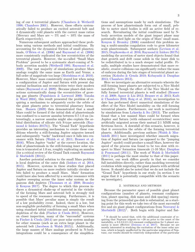
We first evolve the gas giants (without terrestrial plan-ets or a exterior disk of planetesimals) using the Mer-cury6 Bulirsch-Stoer integrator (as opposed to the fasterhybrid integrator) with a 6.0 day timestep (Chambers1999; Stoer et al. 2002). The Bulirish-Stoer method isnecessary when building resonant configurations becausethe force on a particle is a function of both the posi-tions and momenta (Chambers 1999; Batygin & Brown2010b). The planets are initially placed on orbits justoutside their respective resonances, and then integrateduntil the outermost planet’s semi-major axis is at the ap-propriate location (table 1). Figure 1 shows an exampleof this evolution for a simulation in the n1 batch. Toverify that the planets are in a MMR, libration about aseries of resonant angles is checked for using the methoddescribed in Clement & Kaib (2017).

After the resonant chain is assembled, we add a disk

ice giant resonant configuration selected.

of 1000 equal massed planetesimals using the inner andouter radii that Nesvorny & Morbidelli (2012) showedbest meet dynamical constraints for the outer solar sys-tem (table 1). The orbital distribution of the planetesi-mals is chosen in a manner consistent with previous au-thors (Batygin & Brown 2010b; Nesvorny & Morbidelli2012; Kaib & Chambers 2016), and follows an r−1 sur-face density profile. Angular orbital elements (argumentsof pericenter, longitudes of ascending node and meananomalies) for the planetesimals are selected randomly.Eccentricities and inclinations are drawn from near circu-lar and co-planar gaussian distributions (standard devia-tions: σe = .002 and σi = .2◦). These same distributionsare utilized throughout our study to maintain all initialeccentricities less than 0.01, and inclinations within 1◦.These systems are integrated using the Mercury6 hybridintegrator (Chambers 1999) with a 20.0 day timestep upuntil the point when two giant planets first pass within3 mutual Hill Radii. Because we wish to investigate spe-cific instability times with respect to terrestrial planetaryformation, and our resonant configurations can often lastfor tens of millions of years prior to experiencing an insta-bility, we integrate these systems up until the onset of theinstability with an empty inner solar system. Only afterthis point are the terrestrial planetary formation disks atvarious stages of evolution embedded in these systems.The method allows us to save computational time, andcontrol at exactly what point the instability occurs dur-ing the giant impact phase. Though the giant planets arealready on significantly eccentric orbits at this point (andtherefore affecting the terrestrial disk), we find that sys-tems can last for millions of years before experiencing aninstability if the simulation is stopped sooner. Moreover,the terrestrial planets are far more sensitive to the evo-lution of Jupiter and Saturn than that of the ice giants.We find that, in the vast majority of simulations, Jupiterand Saturn don’t begin evolving substantially until af-ter this first close encounter time. In the vast majorityof our simulations, the instability ensues within severalthousand years of the first close-encounter time. Thisis consistent with simulations of planet-planet scatteringdesigned to reproduce giant exoplanet systems (Chatter-jee et al. 2008; Juric & Tremaine 2008; Raymond et al.2010).

Because we want to embed terrestrial planetary disksat different stages of development into a giant planet in-stability, we begin by modeling terrestrial disk evolutionin the presence of a static Jupiter and Saturn in a 3:2MMR. We form 100 systems of terrestrial planets usingthe Mercury6 hybrid integrator (Chambers 1999) and a6.0 day timestep. Because of the integrator’s inabilityto accurately handle low pericenter passages, objects areconsidered to be merged with the sun at 0.1 au (Cham-

5

0.0 0.1 0.2 0.3 0.4 0.5

1.54

1.56

1.58

1.60

1.62

Perio

d R

atio

Saturn:Jupiter

0.0 0.1 0.2 0.3 0.4 0.51.54

1.56

1.58

1.60

1.62

1.64 Ice1:Saturn

0.0 0.1 0.2 0.3 0.4 0.5Time (Myr)

1.481.501.521.541.561.581.601.621.64

Perio

d R

atio

Ice2:Ice1

0.0 0.1 0.2 0.3 0.4 0.5Time (Myr)

1.481.501.521.541.561.581.601.621.641.66 Ice3:Ice2

0.0 0.1 0.2 0.3 0.4 0.50

1

2

3

4

5

6

Res

onan

t Ang

le (r

adia

ns) Saturn:Jupiter

0.0 0.1 0.2 0.3 0.4 0.50

1

2

3

4

5

6Ice1:Saturn

0.0 0.1 0.2 0.3 0.4 0.5Time (Myr)

0

1

2

3

4

5

6

Res

onan

t Ang

le (r

adia

ns) Ice2:Ice1

0.0 0.1 0.2 0.3 0.4 0.5Time (Myr)

0

1

2

3

4

5

6Ice3:Ice2

Figure 1. An example of the resonant evolution of a system ofouter planets in the n1 batch. With the forcing function mimickinginteractions with the gaseous disk in place, once a set of planets fallsin to a MMR, they remain locked in resonance for the remainderof the evolution.

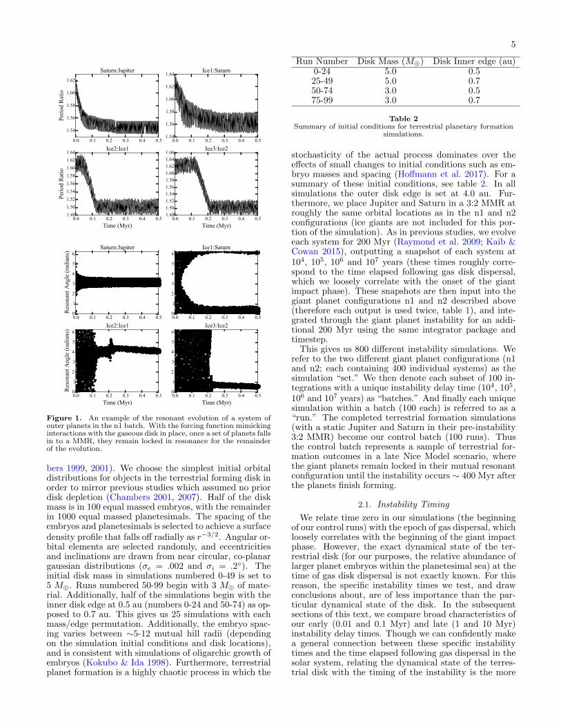
bers 1999, 2001). We choose the simplest initial orbitaldistributions for objects in the terrestrial forming disk inorder to mirror previous studies which assumed no priordisk depletion (Chambers 2001, 2007). Half of the diskmass is in 100 equal massed embryos, with the remainderin 1000 equal massed planetesimals. The spacing of theembryos and planetesimals is selected to achieve a surfacedensity profile that falls off radially as r−3/2. Angular or-bital elements are selected randomly, and eccentricitiesand inclinations are drawn from near circular, co-planargaussian distributions (σe = .002 and σi = .2◦). Theinitial disk mass in simulations numbered 0-49 is set to5 M⊕. Runs numbered 50-99 begin with 3 M⊕ of mate-rial. Additionally, half of the simulations begin with theinner disk edge at 0.5 au (numbers 0-24 and 50-74) as op-posed to 0.7 au. This gives us 25 simulations with eachmass/edge permutation. Additionally, the embryo spac-ing varies between ∼5-12 mutual hill radii (dependingon the simulation initial conditions and disk locations),and is consistent with simulations of oligarchic growth ofembryos (Kokubo & Ida 1998). Furthermore, terrestrialplanet formation is a highly chaotic process in which the

Run Number Disk Mass (M⊕) Disk Inner edge (au)0-24 5.0 0.525-49 5.0 0.750-74 3.0 0.575-99 3.0 0.7

Table 2Summary of initial conditions for terrestrial planetary formation

simulations.

stochasticity of the actual process dominates over theeffects of small changes to initial conditions such as em-bryo masses and spacing (Hoffmann et al. 2017). For asummary of these initial conditions, see table 2. In allsimulations the outer disk edge is set at 4.0 au. Fur-thermore, we place Jupiter and Saturn in a 3:2 MMR atroughly the same orbital locations as in the n1 and n2configurations (ice giants are not included for this por-tion of the simulation). As in previous studies, we evolveeach system for 200 Myr (Raymond et al. 2009; Kaib &Cowan 2015), outputting a snapshot of each system at104, 105, 106 and 107 years (these times roughly corre-spond to the time elapsed following gas disk dispersal,which we loosely correlate with the onset of the giantimpact phase). These snapshots are then input into thegiant planet configurations n1 and n2 described above(therefore each output is used twice, table 1), and inte-grated through the giant planet instability for an addi-tional 200 Myr using the same integrator package andtimestep.

This gives us 800 different instability simulations. Werefer to the two different giant planet configurations (n1and n2; each containing 400 individual systems) as thesimulation “set.” We then denote each subset of 100 in-tegrations with a unique instability delay time (104, 105,106 and 107 years) as “batches.” And finally each uniquesimulation within a batch (100 each) is referred to as a“run.” The completed terrestrial formation simulations(with a static Jupiter and Saturn in their pre-instability3:2 MMR) become our control batch (100 runs). Thusthe control batch represents a sample of terrestrial for-mation outcomes in a late Nice Model scenario, wherethe giant planets remain locked in their mutual resonantconfiguration until the instability occurs ∼ 400 Myr afterthe planets finish forming.

2.1. Instability Timing

We relate time zero in our simulations (the beginningof our control runs) with the epoch of gas dispersal, whichloosely correlates with the beginning of the giant impactphase. However, the exact dynamical state of the ter-restrial disk (for our purposes, the relative abundance oflarger planet embryos within the planetesimal sea) at thetime of gas disk dispersal is not exactly known. For thisreason, the specific instability times we test, and drawconclusions about, are of less importance than the par-ticular dynamical state of the disk. In the subsequentsections of this text, we compare broad characteristics ofour early (0.01 and 0.1 Myr) and late (1 and 10 Myr)instability delay times. Though we can confidently makea general connection between these specific instabilitytimes and the time elapsed following gas dispersal in thesolar system, relating the dynamical state of the terres-trial disk with the timing of the instability is the more

6

important conclusion of our work. As we expand upon inthe subsequent sections, the later two instability delayswe test tend to be more successful than the earlier ones.Therefore our work correlates the giant planet instabilitytiming with a terrestrial disk at a state of evolution thatis mostly depleted of small planetesimals, with most ofthe mass concentrated in a handful of growing planet em-bryos. Subsequently overlaying this timeline on that ofMars’ growth inferred from isotopic dating (Dauphas &Pourmand 2011) is difficult because the relationship be-tween gas disk dispersal and CAI (Calcium-Aluminum-rich inclusion) formation is not well known.

Furthermore, Marty et al. (2017) presented evidencethat cometary bombardment accounted for ∼ 22% of thenoble gas concentration in Earth’s atmosphere. At firstglance, this constraint appears to be slightly at odds withthe various delay times we examine in this paper (0.01-10Myr). We choose to discuss this here in detail becauseit can potentially be construed to undermine the meritof our study. Because the noble gas makeup of the man-tle is so different from that of the atmosphere, and thatof comet 67P, this seems to imply that the onslaughtof comets (the timing of which would correlate with thegiant planet instability) occurred after the moon form-ing impact. Because the moon forming impact occurredafter Mars had completed forming (Kleine et al. 2009;Dauphas & Pourmand 2011), the giant planet instabil-ity could not be the mass-depleting event in the Marsforming region. However this argument does not takein to account the timing of impacts with respect to theEarth’s magma ocean phase. It is reasonable to assumethat some cometary delivery must have occurred prior tocore closure. If fractionalization of Xenon occurred dur-ing the magma ocean phase, the preserved signature inthe mantle could very well be different from that in theatmosphere. Because neither the distribution of impacttimes of primordial Kuiper belt objects (KBOs), nor thefractionalization of Xenon in the magma ocean are wellknown, drawing a broad conclusion of the timing of theinstability from this constraint is difficult. Additionally,delivery itself may have been stochastic; in that an earlyinstability might set the Xenon content of the mantle bydelivering many small comets, and then a later impact ofa large comet could boost the Xenon fraction in the atmo-sphere. Finally, Xenon isotope trends are not well knownover a large enough sample of comets. It is reasonableto expect that comet 67P’s specific Xenon concentrationwould fall somewhere on a continuum when comparedto other similar comets. A larger sample of such mea-surements must be made before these conclusions can beapplied to the giant planet instability timeline. There-fore, as a starting point for our study, we argue that themost important constraint for instability timing is thesurvivability of the terrestrial planets, which no scenarioto date can ensure.

3. SUCCESS CRITERIA

When analyzing the results of our simulations, the pa-rameter space for comparison to the actual solar systemis extensive. Furthermore, for many metrics our accuracyis strongly limited by the resolution of our simulations.For example, the planetary embryos used in the major-ity of our simulations begin the integration with a fourthof Mars’ present mass. Therefore, a “successful” Mars

analog could be formed from as few as 2-3 impacts. Forthese reasons our criteria must be broad, because we aremore interested in looking at statistical consistencies andorder of magnitude agreements than perfectly replicatingevery nuance of the actual solar system. Thus, we focuson 10 broad criteria for replication of both the inner andouter solar systems, which we summarize in table 3.

3.1. The Inner Solar System

Because our goal is to look for systems like our own,with particular emphasis on forming Mars analogs, weemploy an analysis metric similar to Chambers (2001).A system is considered to meet criterion A if it formsa Mars sized body in the vicinity of Mars’ semi-majoraxis, exterior to two Earth sized bodies. We first checkfor any planets formed in the region of 1.3-2.0 au, wherethe inner edge of this region is roughly equal to Mars’current pericenter (∼1.38 au) and the outer limit liesat the inner edge of the asteroid belt. If this planethas a mass less than 0.3 M⊕, is immediately exteriorto two planets each with masses greater than 0.6 M⊕,and the system contains no planets greater than 0.3 M⊕in the asteroid belt, criterion A is satisfied. A separatesuccess criteria (criterion D, section 3.3) filters out sys-tems that finish with an embryo in the Asteroid Beltas unsuccessful. While some authors (Hansen 2009) se-lect 0.2 M⊕ as the upper mass limit for Mars analogs,due to the previously discussed resolution limitation en-countered when using 0.025 M⊕ embryos, we follow theprescription in Raymond et al. (2009) and use 0.3 M⊕as our limit. Additionally, because our simulations donot take collisional fragmentation in to account (for fur-ther discussion of this phenomenon, see section 5.6), it ispossible that the masses of our Mars analogs are some-what over-estimated. Because we set the Venus/Earthminimum mass to 0.6 M⊕ (approximately 75% that ofVenus’ present mass), this provides an adequate massdisparity of a factor of 2 between the Venus/Earth andMars analogs. We also look at systems which form threeplanets of the correct mass (criterion A1), but do nothave the correct semi major axes (eg: Mars formed ata semi-major axis greater than 2.0 au). For this crite-rion, we include systems which form no Mars, but doaccrete appropriately sized Earth and Venus analogs inthe correct locations as being successful.

3.2. The Formation Timescales of Earth and Mars

Mars is often thought to have been left behind as a“stranded embryo” (Morbidelli et al. 2000) during theprocess of planetary formation because the timescale forits accretion inferred from Hf/W dating (.1-10 Myr) isso quick (Nimmo & Agnor 2006; Dauphas & Pourmand2011). Contrarily, Earth is believed to have formed muchslower; of order 50-150 Myr (Touboul et al. 2007; Kleineet al. 2009). There is a significant amount of uncertaintyin both of these timescales. The specific timing of themoon forming impact, which is thought to correlate withthe last major accretion event on Earth, is still not wellknown. Unfortunately, these metrics are quite difficultto meet when using standard embryo accretion numeri-cal models. In fact, planets with semi-major axes greaterthan 1.3 au in our control simulation (which assume nogas giant evolution) almost always form far slower than

7

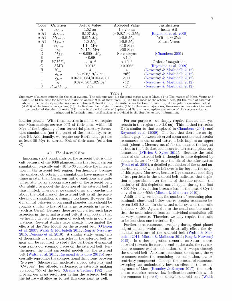
Code Criterion Actual Value Accepted Value JustificationA aMars 1.52 au 1.3-2.0 au Inside AB

A,A1 MMars 0.107 M⊕ > 0.025, < .3M⊕ (Raymond et al. 2009)A,A1 MV enus 0.815 M⊕ >0.6 M⊕ Within ∼ 25%A,A1 MEarth 1.0 M⊕ >0.6 M⊕ Match Venus

B τMars 1-10 Myr <10 MyrC τ⊕ 50-150 Myr >50 MyrD MAB ∼ 0.0004 M⊕ No embryos (Chambers 2001)E ν6 ∼0.09 <1.0F WMF⊕ ∼ 10−3 > 10−4 Order of magnitudeG AMD 0.0018 <0.0036 (Raymond et al. 2009)H NGP 4 4 (Nesvorny & Morbidelli 2012)I aGP 5.2/9.6/19/30au 20% (Nesvorny & Morbidelli 2012)I eGP 0.046/0.054/0.044/0.01 <.11 (Nesvorny & Morbidelli 2012)I iGP 0.37/0.90/1.02/.67◦ < 2◦ (Nesvorny & Morbidelli 2012)J PSat/PJup 2.49 <2.8 (Nesvorny & Morbidelli 2012)

Table 3Summary of success criteria for the solar system. The columns are: (1) the semi-major axis of Mars, (2-4) The masses of Mars, Venus and

Earth, (5-6) the time for Mars and Earth to accrete 90% of their mass, (7) the final mass of the asteroid belt, (8) the ratio of asteroidsabove to below the ν6 secular resonance between 2.05-2.8 au, (8) the water mass fraction of Earth, (9) the angular momentum deficit(AMD) of the inner solar system, (10) the final number of giant planets, (11-13) the semi-major axes, time-averaged eccentricities and

inclination of the giant planets, (14) the orbital period ratio of Jupiter and Saturn. A complete discussion of the success criteria,background information and justifications is provided in the Supplementary Information.

interior planets. With these metrics in mind, we requireour Mars analogs accrete 90% of their mass within 10Myr of the beginning of our terrestrial planetary forma-tion simulations (not the onset of the instability, crite-rion B). Additionally, we require our Earth analogs takeat least 50 Myr to accrete 90% of their mass (criterionC)

3.3. The Asteroid Belt

Imposing strict constraints on the asteroid belt is diffi-cult because, of the 1000 planetesimals that begin a givensimulation, typically only 10 to 30 complete the integra-tion in the asteroid belt region. Furthermore, becausethe smallest objects in our simulations have masses ∼16times greater than Ceres, our initial conditions are quiteunrealistic for an appropriate study of the asteroid belt.Our ability to model the depletion of the asteroid belt isthus limited. Therefore, we cannot draw any conclusionsabout the total mass of the asteroid belt as all the parti-cles in our simulation are simply too large. However, thedynamical behavior of our small planetesimals should beroughly similar to that of the larger asteroids in the belt(such as Ceres). Because there are only a few such largeasteroids in the actual asteroid belt, it is important thatwe heavily deplete the region of such objects in our sim-ulations. Several studies have already investigated theeffects of the Nice Model on the asteroid belt (O’Brienet al. 2007; Walsh & Morbidelli 2011; Roig & Nesvorny2015; Deienno et al. 2016). A similar study, using tensof thousands of smaller particles in the asteroid belt re-gion will be required to study the particular dynamicalconstraints our scenario places on the asteroid belt. Fur-thermore, the most successful models for the asteroidbelt (Walsh et al. 2011; Raymond & Izidoro 2017b) suc-cessfully reproduce the compositional dichotomy between“S-types” (Silicate rich, moderate albedo asteroids) and“C-types” (low albedo, carbonaceous asteroids makingup about 75% of the belt) (Gradie & Tedesco 1982). Im-proving our mass resolution within the asteroid belt inthe future will allow us to test this constraint as well.

For our purposes, we simply require that no embryosremain in the region (a > 2.0 au). This method (criterionD) is similar to that employed in Chambers (2001) andRaymond et al. (2009). The fact that there are no sig-nificant gaps between observed mean motion and secularresonances in the actual asteroid belt implies an upperlimit (about a Mercury mass) for the mass of the largestobject in the belt that could survive terrestrial planetaryformation (O’Brien & Sykes 2011). Because the totalmass of the asteroid belt is thought to have depleted byabout a factor of ∼ 104 over the life of the solar system(Petit et al. 2001), a detailed calculation of the actual nu-merical value of what is left over is far beyond the scopeof this paper. Moreover, because Gyr timescale modelingof test particles in the asteroid belt indicates that deple-tion is logarithmic over the life of the solar system, themajority of this depletion must happen during the first∼200 Myr of evolution because loss in the next 4 Gyr isonly of order ∼50% (Minton & Malhotra 2010).

Additionally, we look at the number of remaining plan-etesimals above and below the ν6 secular resonance be-tween 2.05-2.8 au. In the actual solar system, this ratiois about ∼ .09. Again, due to the small number statis-tics, the ratio inferred from an individual simulation willbe very imprecise. Therefore we only require this ratioto be less than one (criterion E).

Furthermore, resonance sweeping during giant planetmigration and evolution can drastically effect the dy-namical structure of the asteroid belt (Walsh & Mor-bidelli 2011; Minton & Malhotra 2011; Roig & Nesvorny2015). In a slow migration scenario, as Saturn movesoutward towards its current semi-major axis, the ν16 sec-ular resonance excites inclinations as it sweeps throughthe asteroid belt. As Saturn continues to migrate, the ν6resonance erodes the remaining low inclination, low ec-centricity component. Though the process of resonancesweeping can undoubtedly have an effect on the result-ing mass of Mars (Bromley & Kenyon 2017), the mech-anism can also remove low inclination asteroids whichare common (figure 6) in today’s asteroid belt (Walsh

8

& Morbidelli 2011). To preserve the structure of theasteroid belt from the effects of resonance dragging, pre-vious authors (Roig & Nesvorny 2015) utilized a “jump-ing Jupiter” model instability (wherein Jupiter and Sat-urn “jump” toward their present orbital locations, ide-ally preserving the fragile terrestrial planets and asteroidbelt structure). In order for our model to be successful,it must heavily deplete the asteroid belt while still main-taining the low inclination component.

3.4. Water Delivery to Earth

Many models trace the origin of Earth’s water to theearly depletion of the primordial asteroid belt (Raymondet al. 2007, 2009). The actual topic of water delivery toEarth is extensive, with many competing models, andfar beyond the scope of this paper (for a more completediscussion of various ideas see Morbidelli et al. (2000),Morbidelli et al. (2012) and Marty et al. (2016)). Un-certainties in the initial disk properties and locations ofvarious snow lines make it challenging for embryo ac-cretion models like our own to confidently quantify thewater mass fraction (WMF) of Earth analogs. In addi-tion, the actual bulk water content of Earth is extremelyuncertain. Estimates of the mantle’s water content rangebetween 0 to tens of oceans (Lecuyer et al. 1998; Marty2012; Halliday 2013), awhile the core may contain 0 tonearly 100 (Badro 2014; Nomura et al. 2014). See the re-view by Hirschmann (2006) for a discussion of the differ-ence between the capacity of Earth’s water reservoirs andgeochemical evidence for the actual water contained inEarth’s interior. Furthermore, given the amount of plan-etesimal scattering which occurs when the giant plan-ets grew and migrated during the gas disk phase, thematerial from which Earth formed during the giant im-pact phase may have already been sufficiently water rich(Raymond & Izidoro 2017a). For our simulations, wefirst look at the bulk WMF of Earth analogs calculatedusing an initial water radial distribution similar to thatused in Raymond et al. (2009) (equation 1, this assumesthat the primordial asteroid belt region was populatedby water-rich objects from the outer solar system duringthe gas disk phase (Raymond & Izidoro 2017a)). Anysystem which boosts Earth’s WMF to greater than 10−4

is considered to satisfy criterion F. We also analyze thepercentage of objects Earth analogs accrete from differ-ent sections of the disk.

WMF =

10−5, r < 2au

10−3, 2au < r < 2.5au

10%, r > 2.5au

(1)

3.5. Angular Momentum Deficit

One defining aspect about our solar system is the re-markably low eccentricities and inclinations of the terres-trial planets. Over lengthy integrations, the orbits of allthe inner planets but Mercury typically stay extremelylow (Quinn et al. 1991; Laskar & Gastineau 2009). Thisorbital constraint was very difficult for early accretionmodels to meet (Chambers & Wetherill 1998; Chambers2001). O’Brien et al. (2006) used dynamical friction toexplain how the orbits could stay cold through the stan-dard process of planetary formation. However, it hasproven even more challenging to keep eccentricities low

when a giant planet instability is considered (Brasseret al. 2009; Kaib & Chambers 2016). Any successfulmodel of terrestrial planetary formation must maintainlow orbital excitation in the inner solar system. To mea-sure this in our systems, we measure the angular momen-tum deficit (AMD, criterion F) of each system (Laskar1997). AMD (equation 2) quantifies the deviation of theorbits in a system from perfectly coplanar, circular or-bits. We follow the same procedure as Raymond et al.(2009) and require our systems maintain an AMD lessthan twice the value of the modern inner solar system(∼.0018).

AMD =

∑imi√ai[1−

√(1− e2i ) cos ii]∑

imi√ai

(2)

3.6. The Outer Solar System

When analyzing the success of our terrestrial plane-tary formation simulations, it is important to considerhow dependent our results are on the fate of the outersolar system. Indeed, the chance of our chosen resonantchains reproducing all the important traits of the outersolar system after undergoing an instability is often low.For example, Nesvorny & Morbidelli (2012) report onlya 33% chance of our n1 configurations finishing the inte-gration with the correct number of outer planets. Whenall four success criteria in that work are considered, n1resonant chains only successfully match the outer solarsystem ∼ 4% of the time. Given the computational costof our integrations, we are less interested in how oftenwe correctly replicate the orbital architecture of the gi-ant planets, and more concerned with how dependent ourresults are on the fate of the outer solar system.

To quantify the outer solar system, we adopt the samesuccess criteria as Nesvorny & Morbidelli (2012). First,criterion H requires that the simulation finish with 4 gi-ant planets. If this is satisfied, criterion I stipulates thatthe final semi-major axis of each planet be within 20%of the modern location, and the time averaged eccen-tricity and inclination of each planet be less than twicethe largest current value in the outer solar system. Fi-nally, criterion J states that the period ratio of Jupiterand Saturn stay less than 2.8. It should be noted that,unlike Nesvorny & Morbidelli (2012), we check for crite-rion J independently of whether the other two standardsare met. The dynamics of the forming terrestrial plan-ets are far less sensitive to the behavior of the ice giantsthan they are to that of Jupiter and Saturn. Therefore,we are nearly just as interested in systems that correctlyproduce Jupiter and Saturn but eject too many ice giantsas we are in those that replicate the outer solar systemperfectly.

4. RESULTS AND DISCUSSION

We provide complete summaries of our results in tables4, 5 and 6. It should be noted that a small number of ourinstabilities fail to properly eject an ice giant, and com-plete the integration with greater than four giant planets.Because we are only interested in systems similar to thesolar system, we do not include these few outliers in anyof our analyses. Table 4 shows the total percentage ofsystems in each simulation batch which meet our successcriteria for the inner solar system. Table 5 summarizes

9

Set A A1 B C D E F Ga,mTP mTP τmars τ⊕ MAB ν6 WMF AMD

Control 0 0 9 86 2 53 87 8n1/.01Myr 3 15 31 84 41 35 40 14n2/.01Myr 2 6 15 75 48 46 34 9n1/.1Myr 0 2 16 79 38 39 27 12n2/.1Myr 6 10 20 69 50 39 38 12n1/1Myr 13 13 6 90 38 31 47 13n2/1Myr 8 14 11 87 54 42 44 7n1/10Myr 12 20 3 73 48 26 47 16n2/10Myr 8 20 19 80 54 31 62 8

Table 4Summary of percentages of systems which meet the various terrestrial planet success criteria established in table 3. It should be noted

that, because runs beginning with a disk mass of 3M⊕ were not successful at producing appropriately massed Earth and Venus analogs,criterion A and A1 are only calculated for 5M⊕ systems. The subscripts TP and AB indicate the terrestrial planets and asteroid belt

respectively.

Set H I JNGP a,e,iGP S:J

n1/.01Myr 27 14 47n2/.01Myr 18 6 41n1/.1Myr 14 7 42n2/.1Myr 18 3 38n1/1Myr 23 15 57n2/1Myr 22 9 38n1/10Myr 17 9 36n2/10Myr 16 8 36

Table 5Summary of percentages of systems which meet the various giantplanet success criteria established in table 3. The subscript GP

indicates the giant planets.

the percentage of systems satisfying our giant planet suc-cess criteria. We find that our systems adequately repli-cate the outer solar system with frequencies consistentwith those reported in Nesvorny & Morbidelli (2012). Intable 6, we look at our success rates for systems withJupiter/Saturn configurations most similar to the actualsolar system (period ratios less than 2.8). Clearly, thefate of the terrestrial planets is highly dependent on theevolution of the solar system’s two giant planets. This islargely due to strong secular perturbations which resultfrom the post-instability excitation of the giant planetorbits. Indeed, when we look at systems which eject allice giants and finish with a highly eccentric Jupiter andSaturn outside a period ratio of 2.8, we find terrestrialplanets which are too few in number, on excited orbitsand systematically under-massed. Though we still seethese symptoms in some of the systems summarized intable 6, they are noticeably less frequent.

4.1. Formation of a Small Mars

An early instability is highly successful at producinga small Mars, regardless of instability timing and theparticular evolution of the giant planets. 75% of all ourinstability systems form either no Mars or a small Mars(less than 0.3 M⊕), as opposed to none of our controlruns. Additionally, as shown in table 4, most of our con-trol systems leave at least one embryo in the asteroidbelt. In fact, many of these systems even form multiplesmall planets, or an Earth massed planet in the aster-oid belt. Only 9% of our instability simulations forma planet more massive than Mars in the asteroid belt,as opposed to 65% of our control runs. Clearly a Nice

10-1 100

MMars (M⊕)

0.0

0.2

0.4

0.6

0.8

1.0

Cum

ulat

ive

Frac

tion

of M

ars A

nalo

gs

InstabilityControl

Figure 2. Cumulative distribution of Mars analog masses formedin instability systems and our control batch (note that some sys-tems form multiple planets in this region, here we only plot thelargest planet). The vertical line corresponds to Mars’ actual mass.All control runs with a Mars analog smaller than 0.3 M⊕ (∼20%of the batch) were unsuccessful in that they also formed a largeplanet in the asteroid belt

Model instability is a highly efficient means of depletingthe planetesimal disk region of material outside of 1.3 au.

Figure 2 shows the cumulative distribution of thelargest planets in each system formed between 1.3 and2.0 au for our instability sets versus the control batch.The solar system fits in well with this distribution, withslightly greater than half of our systems forming Marsanalogs larger than the actual planet. Indeed, the in-stability consistently starves this region of material andproduces a small planet. In fact, 22% of our systems pro-duce no planet in the Mars region whatsoever. This isslightly lower for the two earliest instability delays (0.01and 0.1 Myr) which we test, with 18% of such systemsforming no Mars in the 1.3 to 2.0 au region. This is dueto the fact that, when the instability occurs, the ratioof the number of planetesimals to embryos, and that oftotal planetesimal mass to total embryo mass is muchhigher. In the late instability cases, the majority of thesystem mass is trapped in several large embryos. Thedynamical excitement of the additional planetesimals inthe early instability delay cases allows the disk mass todisperse, thereby enhancing the mass of Mars analogs.

10

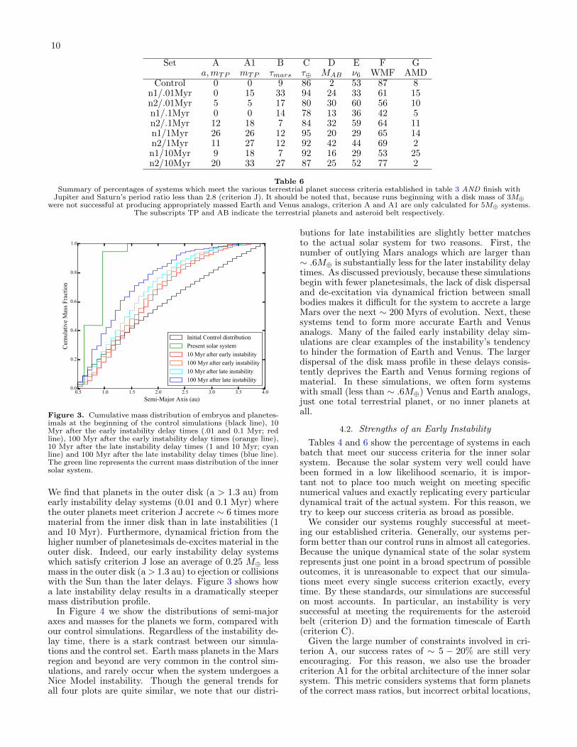
Set A A1 B C D E F Ga,mTP mTP τmars τ⊕ MAB ν6 WMF AMD

Control 0 0 9 86 2 53 87 8n1/.01Myr 0 15 33 94 24 33 61 15n2/.01Myr 5 5 17 80 30 60 56 10n1/.1Myr 0 0 14 78 13 36 42 5n2/.1Myr 12 18 7 84 32 59 64 11n1/1Myr 26 26 12 95 20 29 65 14n2/1Myr 11 27 12 92 42 44 69 2n1/10Myr 9 18 7 92 16 29 53 25n2/10Myr 20 33 27 87 25 52 77 2

Table 6Summary of percentages of systems which meet the various terrestrial planet success criteria established in table 3 AND finish with

Jupiter and Saturn’s period ratio less than 2.8 (criterion J). It should be noted that, because runs beginning with a disk mass of 3M⊕were not successful at producing appropriately massed Earth and Venus analogs, criterion A and A1 are only calculated for 5M⊕ systems.

The subscripts TP and AB indicate the terrestrial planets and asteroid belt respectively.

0.5 1.0 1.5 2.0 2.5 3.0 3.5 4.0Semi-Major Axis (au)

0.0

0.2

0.4

0.6

0.8

1.0

Cum

ulat

ive

Mas

s Fra

ctio

n

Initial Control distributionPresent solar system10 Myr after early instability100 Myr after early instability10 Myr after late instability100 Myr after late instability

Figure 3. Cumulative mass distribution of embryos and planetes-imals at the beginning of the control simulations (black line), 10Myr after the early instability delay times (.01 and 0.1 Myr; redline), 100 Myr after the early instability delay times (orange line),10 Myr after the late instability delay times (1 and 10 Myr; cyanline) and 100 Myr after the late instability delay times (blue line).The green line represents the current mass distribution of the innersolar system.

We find that planets in the outer disk (a > 1.3 au) fromearly instability delay systems (0.01 and 0.1 Myr) wherethe outer planets meet criterion J accrete ∼ 6 times morematerial from the inner disk than in late instabilities (1and 10 Myr). Furthermore, dynamical friction from thehigher number of planetesimals de-excites material in theouter disk. Indeed, our early instability delay systemswhich satisfy criterion J lose an average of 0.25 M⊕ lessmass in the outer disk (a> 1.3 au) to ejection or collisionswith the Sun than the later delays. Figure 3 shows howa late instability delay results in a dramatically steepermass distribution profile.

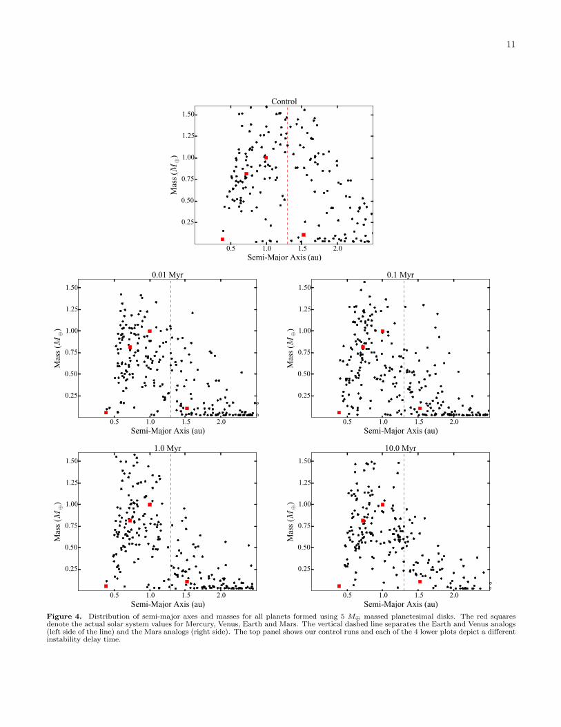
In Figure 4 we show the distributions of semi-majoraxes and masses for the planets we form, compared withour control simulations. Regardless of the instability de-lay time, there is a stark contrast between our simula-tions and the control set. Earth mass planets in the Marsregion and beyond are very common in the control sim-ulations, and rarely occur when the system undergoes aNice Model instability. Though the general trends forall four plots are quite similar, we note that our distri-

butions for late instabilities are slightly better matchesto the actual solar system for two reasons. First, thenumber of outlying Mars analogs which are larger than∼ .6M⊕ is substantially less for the later instability delaytimes. As discussed previously, because these simulationsbegin with fewer planetesimals, the lack of disk dispersaland de-excitation via dynamical friction between smallbodies makes it difficult for the system to accrete a largeMars over the next ∼ 200 Myrs of evolution. Next, thesesystems tend to form more accurate Earth and Venusanalogs. Many of the failed early instability delay sim-ulations are clear examples of the instability’s tendencyto hinder the formation of Earth and Venus. The largerdispersal of the disk mass profile in these delays consis-tently deprives the Earth and Venus forming regions ofmaterial. In these simulations, we often form systemswith small (less than ∼ .6M⊕) Venus and Earth analogs,just one total terrestrial planet, or no inner planets atall.

4.2. Strengths of an Early Instability

Tables 4 and 6 show the percentage of systems in eachbatch that meet our success criteria for the inner solarsystem. Because the solar system very well could havebeen formed in a low likelihood scenario, it is impor-tant not to place too much weight on meeting specificnumerical values and exactly replicating every particulardynamical trait of the actual system. For this reason, wetry to keep our success criteria as broad as possible.

We consider our systems roughly successful at meet-ing our established criteria. Generally, our systems per-form better than our control runs in almost all categories.Because the unique dynamical state of the solar systemrepresents just one point in a broad spectrum of possibleoutcomes, it is unreasonable to expect that our simula-tions meet every single success criterion exactly, everytime. By these standards, our simulations are successfulon most accounts. In particular, an instability is verysuccessful at meeting the requirements for the asteroidbelt (criterion D) and the formation timescale of Earth(criterion C).

Given the large number of constraints involved in cri-terion A, our success rates of ∼ 5 − 20% are still veryencouraging. For this reason, we also use the broadercriterion A1 for the orbital architecture of the inner solarsystem. This metric considers systems that form planetsof the correct mass ratios, but incorrect orbital locations,

11

0.5 1.0 1.5 2.0Semi-Major Axis (au)

0.25

0.50

0.75

1.00

1.25

1.50

Mas

s (M

⊕)

Control

0.5 1.0 1.5 2.0Semi-Major Axis (au)

0.25

0.50

0.75

1.00

1.25

1.50

Mas

s (M

⊕)

0.01 Myr

0.5 1.0 1.5 2.0Semi-Major Axis (au)

0.25

0.50

0.75

1.00

1.25

1.50M

ass (M

⊕)

0.1 Myr

0.5 1.0 1.5 2.0Semi-Major Axis (au)

0.25

0.50

0.75

1.00

1.25

1.50

Mas

s (M

⊕)

1.0 Myr

0.5 1.0 1.5 2.0Semi-Major Axis (au)

0.25

0.50

0.75

1.00

1.25

1.50

Mas

s (M

⊕)

10.0 Myr

Figure 4. Distribution of semi-major axes and masses for all planets formed using 5 M⊕ massed planetesimal disks. The red squaresdenote the actual solar system values for Mercury, Venus, Earth and Mars. The vertical dashed line separates the Earth and Venus analogs(left side of the line) and the Mars analogs (right side). The top panel shows our control runs and each of the 4 lower plots depict a differentinstability delay time.

12

0.0

0.1

0.2

0.3t=0: Dispersal of the gas disk.

0.0

0.1

0.2

0.3t=10 Myr: The instability istriggered.

0.0

0.1

0.2

0.3

Ecce

ntric

ity

t=20 Myr: Mars growthcomplete. Earth and Venusstill forming.

0.0

0.1

0.2

0.3t=210 Myr: Final state of thesystem.

1 10Semi-Major Axis (au)

0.0

0.1

0.2

0.3

0.4Present Solar System.

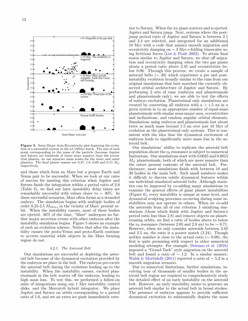
Figure 5. Semi-Major Axis/Eccentricity plot depicting the evolu-tion of a successful system in the n1/10Myr batch. The size of eachpoint corresponding to the mass of the particle (because Jupiterand Saturn are hundreds of times more massive than the terres-trial planets, we use separate mass scales for the inner and outerplanets). The final planet masses are 0.37, 1.0, 0.69 and 0.15 M⊕respectively.

and those which form no Mars but a proper Earth andVenus pair to be successful. When we look at our ratesof success for meeting this criterion when Jupiter andSaturn finish the integration within a period ratio of 2.8(Table 6), we find our later instability delay times areremarkably successful with values closer to ∼ 30%. Inthese successful scenarios, Mars often forms as a strandedembryo. The simulation begins with multiple bodies oforder 0.25-2.5 MMars in the vicinity of Mars’ present or-bit. When the instability ensues, most of these bodiesare ejected. 40% of the time, “Mars” undergoes no fur-ther major accretion events with other embryos after theinstability simulation begins. Figure 5 shows an exampleof such an evolution scheme. Notice that after the insta-bility ensues the proto-Venus and proto-Earth continueto accrete material while objects in the Mars formingregion do not.

4.2.1. The Asteroid Belt

Our simulations are successful at depleting the aster-oid belt because of the dynamical excitation provided bythe embryos we place in the belt. The embryos pre-excitethe asteroid belt during the evolution leading up to theinstability. When the instability ensues, excited plan-etesimals in the belt scatter off the embryos, leading tohigh mass loss. To test this, we performed a follow-onsuite of integrations using our 1 Myr instability controldisks, and the Mercury6 hybrid integrator. We placeJupiter and Saturn on orbits corresponding to a periodratio of 1.6, and set an extra ice giant immediately exte-

rior to Saturn. When the ice giant scatters and is ejected,Jupiter and Saturn jump. Next, systems where the post-jump period ratio of Jupiter and Saturn is between 2.1and 2.4 are selected, and integrated for an additional10 Myr with a code that mimics smooth migration andeccentricity damping on ∼ 3 Myr e-folding timescales us-ing fictitious forces (Lee & Peale 2002). To attain finalstates similar to Jupiter and Saturn, we shut off migra-tion and eccentricity damping when the two gas giantsattain a period ratio above 2.45 and eccentricities be-low 0.06. Through this process, we create a sample ofasteroid belts (∼ 20) which experience a pre and post-instability evolution broadly similar to the runs from ouroriginal simulations that best matched the currently ob-served orbital architecture of Jupiter and Saturn. Byperforming 2 sets of runs (embryos and planetesimalsand planetesimals only), we are able to test the effectsof embryo excitation. Planetesimal only simulations arecreated by converting all embryos with a > 1.5 au in agiven system in to an appropriate number of equal-massplanetesimals with similar semi-major axes, eccentricitiesand inclinations, and random angular orbital elements.Simulations using embryos and planetesimals lost abouttwice as much mass beyond 1.5 au over just 10 Myr ofevolution as the planetesimal only systems. This is con-sistent with the idea that the dynamical excitement ofembryos leads to significantly more mass loss in the as-teroid belt.

Our simulations’ ability to replicate the asteroid beltpopulation about the ν6 resonance is subject to numericallimitations. Our simulations start with 0.0025 and 0.0015M⊕ planetesimals, both of which are more massive thanthe entire present contents of the asteroid belt. Fur-thermore, most simulations finish with between 10 and30 bodies in the main belt. Such small numbers makesit difficult to discern subtle dynamical features withinour individual simulated asteroid belts. Although statis-tics can be improved by co-adding many simulations toexamine the general effects of giant planet instabilities(Figure 6), every instability is unique at some level, anddynamical sculpting processes occurring during some in-stabilities may not operate in others. When we co-addthe asteroids from all of our criterion J satisfying sim-ulations (those which finish with Jupiter and Saturn’speriod ratio less than 2.8) and remove objects on planet-crossing orbits, we find a ratio of bodies above to belowthe ν6 resonance (between 2.05 and 2.8 au) to be ∼ 0.71.However, when we only consider asteroids between 2.05and 2.5 au, the ratio is a poorer match (2.24). Thoughneither number is close to the actual ratio (∼ 0.09), thefirst is quite promising with respect to other numericalmodeling attempts. For example, Deienno et al. (2016)imposed a “Grand-Tack” style migration on the asteroidbelt and found a ratio of ∼ 1.2. In a similar manner,Walsh & Morbidelli (2011) reported a ratio of ∼ 5.2 in asmooth migration scenario.

Due to numerical limitations, further simulations, in-volving tens of thousands of smaller bodies in the as-teroid belt region are required to comprehensively studythe detailed effect of an early instability on the asteroidbelt. However, an early instability seems to generate anasteroid belt similar to the actual belt in broad strokes.The presence of embryos appears to provide sufficientdynamical excitation to substantially deplete the mass

13

0

10

20

30

40

ν6

3:1

5:2

7:3

2:1

AsteroidsMars Crossing

2.0 2.2 2.4 2.6 2.8 3.0 3.2 3.4Semi-Major Axis (au)

0

10

20

30

40

0.0 0.2 0.4 0.6 0.8 1.00.0

0.2

0.4

0.6

0.8

1.0

Incl

inat

ion

(deg

rees

)

Figure 6. The upper plot shows the inclination distribution ofthe modern asteroid belt (only bright objects with absolute mag-nitude H < 9.7, approximately corresponding to D > 50 km, areplotted). The bottom plot combines all planetesimals remaining inthe asteroid belt region from all instability simulations that forma Mars analog less massive than 3 times Mars’ actual mass, andfinish with Jupiter and Saturn’s period ratio less than 2.8. Greypoints correspond to high-eccentricity asteroids on Mars crossingorbits which will be naturally removed during subsequent evolutionup to the solar system’s present epoch. The vertical dashed linesrepresent the locations of the important mean motion resonanceswith Jupiter. The bold dashed lines indicate the current locationof the ν6 secular resonance.

in the region (most simulations deplete more than 95%of belt material in 200 Myr). Though this does fall shortof the required depletion of a factor of ∼ 104 (Petit et al.2001), our mechanism does produce substantial deple-tion in the asteroid belt when compared with our controlruns. More realistic initial conditions and handling ofcollisions will be required to more accurately model de-pletion in the Asteroid Belt in our model. Nevertheless,embryos remaining in the asteroid belt are extremely rarein our instability systems. By using a full instability,rather than a smooth migration scenario, we avoid drag-ging resonances across the belt, thus broadly preservingits orbital structure.

4.3. Weaknesses of an Early Instability

On average, our instability simulations are less suc-cessful at meeting the success criteria for the formationtimescale of Mars, the WMF of Earth and the AMDof the terrestrial planets. Reproducing the formationtimescale of Mars is a difficult constraint for N-body ac-cretion models of terrestrial planetary formation. A suc-cessful Mars analog in our simulations need only be com-posed of 4 embryos. Meanwhile, the real Mars formedfrom millions of smaller objects that accreted prior toand during the giant impact phase. This differencemust be weighed when considering moderate discrepan-cies between the formation timescales of simulated Marsanalogs and the real planet. In fact, ∼ 40% of all ourMars analogs undergo no impacts with other embryosfollowing the instability, and Mars’ form on average ∼ 39Myr faster than their Earth counterparts. Additionally, 6of the 7 Mars analogs in the criterion A1 satisfying [n2/10Myr] batch (our most successful simulations), form inunder 10 Myr. Because Mars’ growth only continued at

the ∼ 10% level after ∼ 2-4 Myr (Dauphas & Pourmand2011), our 1 Myr instability delays are the most suc-cessful at simultaneously matching the mass distributionof the terrestrial system and the proposed accretion his-tory of Mars. However, the geological accretion historyof Mars is inferred relative to CAI formation; the tim-ing relative to gas disk dissipation of which is not fullyunderstood.

Providing a means of water delivery to Earth is not astrict requirement for the success of an embryo accretionmodel. It should be noted that many ideas for how Earthwas populated with water exist, several of which havenothing to do with delivery via bodies from the outersolar system (Morbidelli et al. 2000, 2012). In fact, wa-ter delivering planetesimals may have been scattered onto Earth-crossing orbits during the giant planets’ growthand migration phase (Raymond & Izidoro 2017a). De-spite the small number statistics involved with using only1000 initial particles in the Kuiper belt, about half ofwhich typically deplete in the initial phase of integration(before the terrestrial disks are imbedded), we do find12 instances of Earth analogs accreting objects from thisregion in our simulations. Interestingly, Earth’s noblegases are thought to come primarily from comets, de-spite the fact that comets are likely a minor source ofwater (Marty et al. 2016). We find that a late instabilitydelay time (1 and 10 Myr) systematically stretches thefeeding zone of Earth analogs further in to the terrestrialdisk. This broader feeding zone is basically a result ofeccentricity excitation of planetesimals (Levison & Ag-nor 2003b). In these cases, mass from the outer disk isable to “leap-frog” its way towards the proto-Earth. Inthe first phase of evolution (before the instability), form-ing embryos in the middle part of the disk (∼2.0-3.0 au)accrete material from the outermost section of the disk(∼3.0-4.0 au). When the instability ensues, these em-bryos are destabilized, and occasionally scattered inwardtowards the forming “Earth”.

Our simulations often leave the inner planets with toolarge of an AMD. Though most runs only exceed the ac-tual AMD of the solar system by a factor of 2-3, somesystems occasionally reach AMDs as high as 10 timesthe value of the current solar system. Many of theseoutliers are from integrations where particularity violentinstabilities leave behind a system of overly excited giantplanets. Even when we remove these instances which arenot analogous to the actual solar system, our “success-ful” simulations still tend to possess high AMD values.Often, an overly excited Mars is the source of this or-bital excitation (values of eMars ∼ .1 − .25 are typicalfor these systems). The obvious source of this excita-tion is secular interactions with the excited giant plan-ets. One potential solution to this problem might be ac-counting for collisional fragmentation. Chambers (2013)showed that angular momentum exchange resulting fromhit-and-run collisions noticeably reduces the eccentricityof planets formed in embryo accretion models. Addition-ally, Jacobson & Morbidelli (2014) showed that the AMDof systems increases as the total amount of initial massplaced in embryos instead of planetesimals increases, andas individual embryo mass decreases. We observe a sim-ilar relationship in overall disk mass loss (section 5.1).Moreover, because of the chaotic nature of the actual so-lar system, its AMD can evolve by as much as a factor of

14

2 in either direction over Gyr timescales (Laskar 1997).

4.4. Varied Initial Conditions

Our simulations are broken up into 4 different sets of25 runs with unique inner disk edge and initial disk masscombinations (Table 2). In half of our simulations, we usea disk mass of 3 M⊕ rather than a more typical choice of∼ 5M⊕ (Chambers 2001; Raymond et al. 2009). 100%of these systems with lower mass disks fail to meet crite-rion A for correctly replicating the semi-major axes andmasses of the terrestrial planets. Using a lower overalldisk mass leads to less dynamical friction available tosave bodies from loss after the instability. We find thatby far the most likely final configuration for these simula-tions is a single Venus analog, occasionally accompaniedby a Mars analog. However, we note that the percentagesof systems that meet the other 6 success criteria (crite-rion B through G) are roughly similar (within ∼ 5%) forsystems of either initial disk mass.

We see no noticeable differences between the sets ofsimulations which truncate the inner planetesimal diskat 0.5 au and those with an inner edge at 0.7 au. Bothbatches are roughly equally likely (9% and 10% of thetime, respectively) to form a Mercury analog (we definethis as any planet smaller than 0.2 M⊕ interior to anEarth and a Venus analog). For more discussion on theformation of Mercury, see section 6. Finally, our ratesfor meeting all success criteria for the inner planets areroughly the same (within ∼ 5%), regardless of the se-lected inner disk edge location.

4.5. Excitation of Jupiter’s g5 Mode.

The sufficient excitation of Jupiter’s g5 mode is anotherimportant constraint on the evolution of the giant plan-ets. The current amplitude of the mode, e55 = 0.044,is very important in driving the secular evolution of thesolar system (Morbidelli et al. 2009b). Additionally, theamplitude of Saturn’s forcing on Jupiter’s eccentricity,e56 = 0.016, is important for the long term evolutionof Mars and the asteroid belt. Overexciting e56 mightlead to a small Mars and a depleted asteroid belt. How-ever, this scenario is not akin to the actual evolution ofthe solar system. To evaluate the relationship betweenthe g5 mode and the mass of Mars, we integrate all sys-tems which finish with Jupiter and Saturn within a pe-riod ratio of 2.8 for an additional 10 Myr, and perform aFourier analysis of the additional evolution (Sidlichovsky& Nesvorny 1996). In Figure 7, we plot the values of e55and e56 against the masses of Mars analogs produced forthese systems in our 10 Myr delayed instabilities. Wefind that systems with an e55 amplitude greater thanthat of actual solar system never produce a large Marsanalog (greater than 0.3 M⊕). The average Mars analogmass in systems with e55 less than half the solar sys-tem value (0.022) is 1.96 times Mars’ mass, compared to1.03 for systems with e55 > 0.022. Additionally, we seemultiple examples of systems where e56 is close to thesolar system value, that produce a small Mars. Clearly,the complete excitation of the g5 mode is linked to re-ducing the mass of planets in the Mars forming region.Additionally, in Figure 8, we plot the normalized AMDof Jupiter and Saturn versus the mass of Mars analogs.It is very apparent that the range of possible values is

0.00

0.02

0.04

0.06

Jupi

ter E

xcita

tion

(e55

)

0.0 0.2 0.4 0.6 0.8 1.0MMars (M⊕)

0.00

0.02

0.04

0.06

Satu

rn E

xcita

tion

(e56

)

Figure 7. Values of the amplitudes of Jupiter’s g5 mode versus themass of Mars analogs formed for 10 Myr delayed instability systemswhere the orbital period ratio of Saturn to Jupiter completing theintegration less than 2.8. The red stars correspond with the presentsolar system values.

extensive, with the solar system falling well within therange of our results. Therefore, the actual solar system isconsistent with our dynamical evolution model. Further-more, Jupiter’s excitation also effects Earth and Venus.When we plot the cumulative mass of Earth and Venusagainst the mass of Mars (Figure 9), we find that manyof the systems with similar values to the solar systemhave correspondingly similar values of e55.

4.6. Impact Velocities

Our simulations use an integration scheme whereall collisions are assumed to be perfectly accretionary(Chambers 1999). This provides a decent approxima-tion of the final outcome of terrestrial planet formationfor low relative-velocity collisions between objects witha large mass disparity. However, higher velocity colli-sions can often be erosive (Genda et al. 2012), particu-larly when the projectile to target mass ratio is closerto unity. Additionally, depending on the parameters ofthe impact, glancing blows can lead to the re-accretionof either all, some or none of the original projectile (As-phaug et al. 2006; Asphaug 2010; Stewart & Leinhardt2012). Because of the instability’s tendency to excitesmall planetesimals on to high-eccentricity orbits, the

15

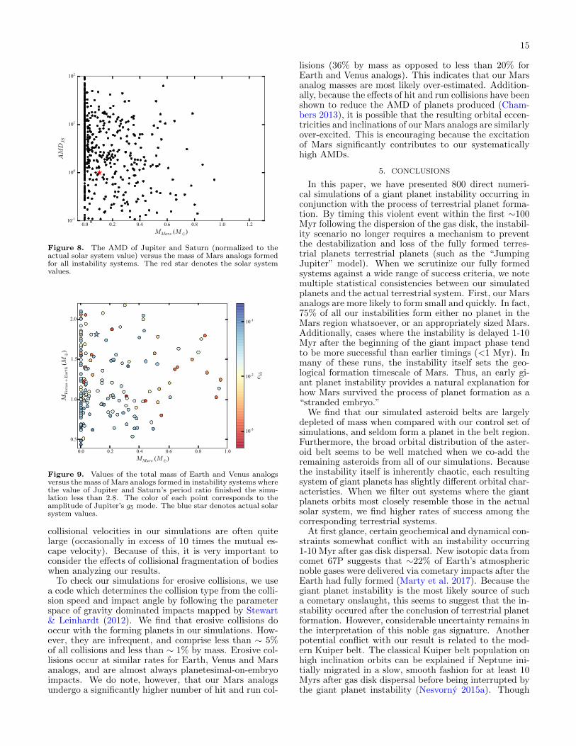
0.0 0.2 0.4 0.6 0.8 1.0 1.2MMars (M⊕)

10-1

100

101

102

AMDJS

Figure 8. The AMD of Jupiter and Saturn (normalized to theactual solar system value) versus the mass of Mars analogs formedfor all instability systems. The red star denotes the solar systemvalues.

0.0 0.2 0.4 0.6 0.8 1.0MMars (M⊕)

0.5

1.0

1.5

2.0

MVenus+Earth (M

⊕)

10-3

10-2

10-1

e 55

Figure 9. Values of the total mass of Earth and Venus analogsversus the mass of Mars analogs formed in instability systems wherethe value of Jupiter and Saturn’s period ratio finished the simu-lation less than 2.8. The color of each point corresponds to theamplitude of Jupiter’s g5 mode. The blue star denotes actual solarsystem values.

collisional velocities in our simulations are often quitelarge (occasionally in excess of 10 times the mutual es-cape velocity). Because of this, it is very important toconsider the effects of collisional fragmentation of bodieswhen analyzing our results.

To check our simulations for erosive collisions, we usea code which determines the collision type from the colli-sion speed and impact angle by following the parameterspace of gravity dominated impacts mapped by Stewart& Leinhardt (2012). We find that erosive collisions dooccur with the forming planets in our simulations. How-ever, they are infrequent, and comprise less than ∼ 5%of all collisions and less than ∼ 1% by mass. Erosive col-lisions occur at similar rates for Earth, Venus and Marsanalogs, and are almost always planetesimal-on-embryoimpacts. We do note, however, that our Mars analogsundergo a significantly higher number of hit and run col-

lisions (36% by mass as opposed to less than 20% forEarth and Venus analogs). This indicates that our Marsanalog masses are most likely over-estimated. Addition-ally, because the effects of hit and run collisions have beenshown to reduce the AMD of planets produced (Cham-bers 2013), it is possible that the resulting orbital eccen-tricities and inclinations of our Mars analogs are similarlyover-excited. This is encouraging because the excitationof Mars significantly contributes to our systematicallyhigh AMDs.

5. CONCLUSIONS

In this paper, we have presented 800 direct numeri-cal simulations of a giant planet instability occurring inconjunction with the process of terrestrial planet forma-tion. By timing this violent event within the first ∼100Myr following the dispersion of the gas disk, the instabil-ity scenario no longer requires a mechanism to preventthe destabilization and loss of the fully formed terres-trial planets terrestrial planets (such as the “JumpingJupiter” model). When we scrutinize our fully formedsystems against a wide range of success criteria, we notemultiple statistical consistencies between our simulatedplanets and the actual terrestrial system. First, our Marsanalogs are more likely to form small and quickly. In fact,75% of all our instabilities form either no planet in theMars region whatsoever, or an appropriately sized Mars.Additionally, cases where the instability is delayed 1-10Myr after the beginning of the giant impact phase tendto be more successful than earlier timings (<1 Myr). Inmany of these runs, the instability itself sets the geo-logical formation timescale of Mars. Thus, an early gi-ant planet instability provides a natural explanation forhow Mars survived the process of planet formation as a“stranded embryo.”

We find that our simulated asteroid belts are largelydepleted of mass when compared with our control set ofsimulations, and seldom form a planet in the belt region.Furthermore, the broad orbital distribution of the aster-oid belt seems to be well matched when we co-add theremaining asteroids from all of our simulations. Becausethe instability itself is inherently chaotic, each resultingsystem of giant planets has slightly different orbital char-acteristics. When we filter out systems where the giantplanets orbits most closely resemble those in the actualsolar system, we find higher rates of success among thecorresponding terrestrial systems.

At first glance, certain geochemical and dynamical con-straints somewhat conflict with an instability occurring1-10 Myr after gas disk dispersal. New isotopic data fromcomet 67P suggests that ∼22% of Earth’s atmosphericnoble gases were delivered via cometary impacts after theEarth had fully formed (Marty et al. 2017). Because thegiant planet instability is the most likely source of sucha cometary onslaught, this seems to suggest that the in-stability occured after the conclusion of terrestrial planetformation. However, considerable uncertainty remains inthe interpretation of this noble gas signature. Anotherpotential conflict with our result is related to the mod-ern Kuiper belt. The classical Kuiper belt population onhigh inclination orbits can be explained if Neptune ini-tially migrated in a slow, smooth fashion for at least 10Myrs after gas disk dispersal before being interrupted bythe giant planet instability (Nesvorny 2015a). Though

16

such a timing matches our longest delay, pushing the in-stability time later leads to a conflict with constraints onMars’ accretion history (Dauphas & Pourmand 2011).However, our understanding of the Kuiper belt’s originsand Mars’ formation timescale are subjects of ongoingstudy and continually evolving. Given this, we believethis is not enough to rule out the premise of our model,especially because it is able to replicate so many featuresof the inner solar system.

The Nice Model explains a number of aspects of theouter solar system. We have shown that, if it occurredwithin 10 Myr of the dissipation of the gaseous disk, theinstability produces inner solar system analogues thatmatch many important observational constraints regard-ing the formation of Mars and the asteroid belt. In con-trast, simulations lacking an instability consistently yieldMars analogs that are too massive, form too slowly, andare surrounded by over-developed asteroid belts. By in-cluding a giant planet instability, these same simulationsshow a dramatic decrease in the mass and formationtimescale of Mars, and adequate depletion in the asteroidbelt.

6. FUTURE WORK

Our simulations are insufficient to study the large scalestructure of the asteroid belt. Simulations utilizing tensof thousands of smaller particles in the asteroid belt arenecessary to test if this model can correctly match theorbital distribution of known asteroids. Additionally, thelarge scale distribution of “S-types” and “C-types” isan important dynamical constraint which must be ac-counted for (Gradie & Tedesco 1982; Bus & Binzel 2002;DeMeo & Carry 2013). Moreover, as our knowledge of as-teroids continues to undoubtedly expand through furthermissions such as Asteroid Redirect, Dawn, OSIRIS-Rexand Lucy, so will the number of constraints.

Another major shortcoming of our project is that wedo not account for the collisional fragmentation of col-liding bodies. Higher velocity collisions can be erosive,rather than accretionary. Given the highly excited orbitswhich are produced by the Nice Model instability in oursimulations, accounting for the fragmentation of bodiesis supremely important. Furthermore, Chambers (2013)showed that accounting for hit-and-run collisions in em-bryo accretion models can result in producing planetson colder orbits than when using standard integrationschemes. Consistent with most previous N-body simula-tions of the late stages of terrestrial planetary formation,our integrations fail to produce Mercury analogs with anyreasonable consistency (Chambers 2001; O’Brien et al.2006; Raymond et al. 2009; Kaib & Cowan 2015). Per-haps accounting for the fragments of material ejected inhigh velocity collisions with Venus analogs might provideinsight into understanding this problem.

Finally, the capture of Mars’ trojan satellites (someof which are rare, olivine-rich “A-type” asteroids) is un-doubtedly affected by the strong excitation of orbits wesee in the proto-Mars region of our simulations (Tabach-nik & Evans 1999). The trojans of Mars are the onlysuch objects in the inner solar system with orbits stableover Gyr timescales. Their unique compositions repre-sent a potential observational constraint for N-body in-tegrations of terrestrial planetary formation (Polishooket al. 2017).

ACKNOWLEDGMENTS

M.S.C. and N.A.K. thank the National Science Foun-dation for support under award AST-1615975. S.N.R.thanks the Agence Nationale pour la Recherche forsupport via grant ANR-13-BS05-0 0 03-0 02 (grantMOJO). K.J.W. thanks NASA’s SSERVI program (In-stitute of the Science of Exploration Targets) throughinstitute grant number NNA14AB03A. The majorityof computing for this project was performed at theOU Supercomputing Center for Education and Research(OSCER) at the University of Oklahoma (OU). Ad-ditional analyses and simulations were done using re-sources provided by the Open Science Grid (Pordeset al. 2007; Sfiligoi et al. 2009), which is supportedby the National Science Foundation award 1148698,and the U.S. Department of Energy’s Office of Sci-ence. Control simulations were managed on the NielsenHall Network using the HTCondor software package:https://research.cs.wisc.edu/htcondor/. This researchis part of the Blue Waters sustained-petascale comput-ing project, which is supported by the National ScienceFoundation (awards OCI-0725070 and ACI-1238993) andthe state of Illinois. Blue Waters is a joint effort ofthe University of Illinois at Urbana-Champaign and itsNational Center for Supercomputing Applications (Bodeet al. 2013; Kramer et al. 2015).

REFERENCES

Agnor, C. B., & Lin, D. N. C. 2012, ApJ, 745, 143Asphaug, E. 2010, Chemie der Erde / Geochemistry, 70, 199Asphaug, E., Agnor, C. B., & Williams, Q. 2006, Nature, 439, 155Badro, J. 2014, Annual Review of Earth and Planetary Sciences,

42, 231Barr, A. C., & Canup, R. M. 2010, Nature Geoscience, 3, 164Baruteau, C., Crida, A., Paardekooper, S.-J., et al. 2014,

Protostars and Planets VI, 667Batygin, K., & Brown, M. E. 2010a, ApJ, 716, 1323—. 2010b, ApJ, 716, 1323Batygin, K., Brown, M. E., & Betts, H. 2012, ApJ, 744, L3Beauge, C., & Nesvorny, D. 2012, ApJ, 751, 119Bode, B., Butler, M., Dunning, T., et al. 2013, in Contemporary

High Performance Computing, Chapman & Hall/CRCComputational Science (Chapman and Hall/CRC), 339–366

Boehnke, P., Harrison, T. M., Heizler, M. T., & Warren, P. H.2016, Earth and Planetary Science Letters, 453, 267

Bottke, W. F., Walker, R. J., Day, J. M. D., Nesvorny, D., &Elkins-Tanton, L. 2010, Science, 330, 1527

Brasser, R., Matsumura, S., Ida, S., Mojzsis, S. J., & Werner,S. C. 2016, ApJ, 821, 75

Brasser, R., Morbidelli, A., Gomes, R., Tsiganis, K., & Levison,H. F. 2009, A&A, 507, 1053

Brasser, R., Walsh, K. J., & Nesvorny, D. 2013, MNRAS, 433,3417

Bromley, B. C., & Kenyon, S. J. 2017, AJ, 153, 216Bus, S. J., & Binzel, R. P. 2002, Icarus, 158, 146Chambers, J. E. 1999, MNRAS, 304, 793—. 2001, Icarus, 152, 205—. 2007, Icarus, 189, 386—. 2013, Icarus, 224, 43Chambers, J. E., & Cassen, P. 2002, Meteoritics and Planetary

Science, 37, 1523Chambers, J. E., & Wetherill, G. W. 1998, Icarus, 136, 304Chapman, C. R., Cohen, B. A., & Grinspoon, D. H. 2007, Icarus,

189, 233Chatterjee, S., Ford, E. B., Matsumura, S., & Rasio, F. A. 2008,

ApJ, 686, 580Clement, M. S., & Kaib, N. A. 2017, Icarus, 288, 88Dauphas, N., & Pourmand, A. 2011, Nature, 473, 489Day, J. M. D., Pearson, D. G., & Taylor, L. A. 2007, Science, 315,

217

17

Deienno, R., Gomes, R. S., Walsh, K. J., Morbidelli, A., &Nesvorny, D. 2016, Icarus, 272, 114

Deienno, R., Morbidelli, A., Gomes, R. S., & Nesvorny, D. 2017,AJ, 153, 153

Delisle, J.-B., Correia, A. C. M., & Laskar, J. 2015, A&A, 579,A128

DeMeo, F. E., & Carry, B. 2013, Icarus, 226, 723Drazkowska, J., Alibert, Y., & Moore, B. 2016, A&A, 594, A105Duncan, M. J., Levison, H. F., & Lee, M. H. 1998, AJ, 116, 2067Fabrycky, D. C., & Murray-Clay, R. A. 2010, ApJ, 710, 1408Fassett, C. I., Head, J. W., Kadish, S. J., et al. 2012, Journal of

Geophysical Research (Planets), 117, E00H06Fernandes, V. A., Burgess, R., & Turner, G. 2000, Meteoritics

and Planetary Science, 35, 1355Fernandez, J. A., & Ip, W.-H. 1984, Icarus, 58, 109Fischer, R. A., & Ciesla, F. J. 2014, Earth and Planetary Science

Letters, 392, 28Genda, H., Kokubo, E., & Ida, S. 2012, ApJ, 744, 137Gomes, R., Levison, H. F., Tsiganis, K., & Morbidelli, A. 2005,

Nature, 435, 466Gomes, R. S. 2003, Icarus, 161, 404Gradie, J., & Tedesco, E. 1982, Science, 216, 1405Grimm, S. L., & Stadel, J. G. 2014, ApJ, 796, 23Hahn, J. M., & Malhotra, R. 1999, AJ, 117, 3041Haisch, Jr., K. E., Lada, E. A., & Lada, C. J. 2001, ApJ, 553,

L153Halliday, A. N. 2008, Philosophical Transactions of the Royal

Society of London Series A, 366, 4163—. 2013, Geochim. Cosmochim. Acta, 105, 146Hansen, B. M. S. 2009, ApJ, 703, 1131Hirschmann, M. M. 2006, Annual Review of Earth and Planetary

Sciences, 34, 629Hoffmann, V., Grimm, S. L., Moore, B., & Stadel, J. 2017,

MNRAS, 465, 2170Holman, M. J., Fabrycky, D. C., Ragozzine, D., et al. 2010,

Science, 330, 51Izidoro, A., Haghighipour, N., Winter, O. C., & Tsuchida, M.

2014, ApJ, 782, 31Izidoro, A., Raymond, S. N., Morbidelli, A., & Winter, O. C.

2015, MNRAS, 453, 3619Jacobson, S. A., & Morbidelli, A. 2014, Philosophical

Transactions of the Royal Society of London Series A, 372, 0174Jacobson, S. A., & Walsh, K. J. 2015, Washington DC American

Geophysical Union Geophysical Monograph Series, 212, 49Juric, M., & Tremaine, S. 2008, ApJ, 686, 603Kaib, N. A., & Chambers, J. E. 2016, MNRAS, 455, 3561Kaib, N. A., & Cowan, N. B. 2015, Icarus, 252, 161Kenyon, S. J., & Bromley, B. C. 2006, AJ, 131, 1837Kleine, T., Touboul, M., Bourdon, B., et al. 2009,

Geochim. Cosmochim. Acta, 73, 5150Kley, W., & Nelson, R. P. 2012, ARA&A, 50, 211Kobayashi, H., & Dauphas, N. 2013, Icarus, 225, 122Kokubo, E., & Genda, H. 2010, ApJ, 714, L21Kokubo, E., & Ida, S. 1998, Icarus, 131, 171Kramer, W., Butler, M., Bauer, G., Chadalavada, K., & Mendes,

C. 2015, in High Performance Parallel I/O, ed. Prabhat &Q. Koziol (CRC Publications, Taylor and Francis Group),17–32

Laskar, J. 1997, A&A, 317, L75Laskar, J., & Gastineau, M. 2009, Nature, 459, 817Lecuyer, C., Grandjean, P., Barrat, J.-A., et al. 1998,

Geochim. Cosmochim. Acta, 62, 2429Lee, M. H., & Peale, S. J. 2002, ApJ, 567, 596Levison, H. F., & Agnor, C. 2003a, AJ, 125, 2692—. 2003b, AJ, 125, 2692Levison, H. F., Kretke, K. A., Walsh, K. J., & Bottke, W. F. 2015,

Proceedings of the National Academy of Science, 112, 14180Levison, H. F., Morbidelli, A., Van Laerhoven, C., Gomes, R., &

Tsiganis, K. 2008, Icarus, 196, 258Lykawka, P. S., & Ito, T. 2013, ApJ, 773, 65Malhotra, R. 1993, Nature, 365, 819—. 1995, AJ, 110, 420Marty, B. 2012, Earth and Planetary Science Letters, 313, 56Marty, B., Avice, G., Sano, Y., et al. 2016, Earth and Planetary

Science Letters, 441, 91Marty, B., Altwegg, K., Balsiger, H., et al. 2017, Science, 356,

1069

Masset, F., & Snellgrove, M. 2001, MNRAS, 320, L55Matsumura, S., Thommes, E. W., Chatterjee, S., & Rasio, F. A.

2010, ApJ, 714, 194Mills, S. M., Fabrycky, D. C., Migaszewski, C., et al. 2016,

Nature, 533, 509Minton, D. A., & Malhotra, R. 2010, Icarus, 207, 744—. 2011, ApJ, 732, 53Minton, D. A., Richardson, J. E., & Fassett, C. I. 2015, Icarus,

247, 172Morbidelli, A., Brasser, R., Gomes, R., Levison, H. F., &

Tsiganis, K. 2010, AJ, 140, 1391Morbidelli, A., Brasser, R., Tsiganis, K., Gomes, R., & Levison,

H. F. 2009a, A&A, 507, 1041—. 2009b, A&A, 507, 1041Morbidelli, A., Chambers, J., Lunine, J. I., et al. 2000,

Meteoritics and Planetary Science, 35, 1309Morbidelli, A., & Crida, A. 2007, Icarus, 191, 158Morbidelli, A., Levison, H. F., Tsiganis, K., & Gomes, R. 2005,

Nature, 435, 462Morbidelli, A., Lunine, J. I., O’Brien, D. P., Raymond, S. N., &

Walsh, K. J. 2012, Annual Review of Earth and PlanetarySciences, 40, 251

Morbidelli, A., Nesvorny, D., Laurenz, V., et al. 2018, Icarus, 305,262

Morbidelli, A., Tsiganis, K., Crida, A., Levison, H. F., & Gomes,R. 2007, AJ, 134, 1790

Morishima, R., Stadel, J., & Moore, B. 2010, Icarus, 207, 517Nesvorny, D. 2011, ApJ, 742, L22—. 2015a, AJ, 150, 73—. 2015b, AJ, 150, 68Nesvorny, D., & Morbidelli, A. 2012, AJ, 144, 117Nesvorny, D., Vokrouhlicky, D., & Morbidelli, A. 2007, AJ, 133,

1962—. 2013, ApJ, 768, 45Nimmo, F., & Agnor, C. B. 2006, Earth and Planetary Science

Letters, 243, 26Nomura, R., Hirose, K., Uesugi, K., et al. 2014, Science, 343, 522O’Brien, D. P., Morbidelli, A., & Bottke, W. F. 2007, Icarus, 191,

434O’Brien, D. P., Morbidelli, A., & Levison, H. F. 2006, Icarus, 184,

39O’Brien, D. P., & Sykes, M. V. 2011, Space Sci. Rev., 163, 41Papaloizou, J. C. B., & Larwood, J. D. 2000, MNRAS, 315, 823Papaloizou, J. C. B., & Nelson, R. P. 2003, MNRAS, 339, 983Pascucci, I., Apai, D., Luhman, K., et al. 2009, ApJ, 696, 143Petit, J.-M., Morbidelli, A., & Chambers, J. 2001, Icarus, 153, 338Pierens, A., & Nelson, R. P. 2008, A&A, 482, 333Polishook, D., Jacobson, S. A., Morbidelli, A., & Aharonson, O.

2017, Nature Astronomy, 1, 0179Pordes, R., Petravick, D., Kramer, B., et al. 2007, Journal of

Physics: Conference Series, 78, 012057Quinn, T. R., Tremaine, S., & Duncan, M. 1991, AJ, 101, 2287Raymond, S. N., Armitage, P. J., & Gorelick, N. 2010, ApJ, 711,

772Raymond, S. N., & Izidoro, A. 2017a, Icarus, 297, 134—. 2017b, Science Advances, 3, e1701138Raymond, S. N., & Morbidelli, A. 2014, in IAU Symposium, Vol.

310, Complex Planetary Systems, Proceedings of theInternational Astronomical Union, 194–203

Raymond, S. N., O’Brien, D. P., Morbidelli, A., & Kaib, N. A.2009, Icarus, 203, 644

Raymond, S. N., Quinn, T., & Lunine, J. I. 2006, Icarus, 183, 265—. 2007, Astrobiology, 7, 66Rivera, E. J., Laughlin, G., Butler, R. P., et al. 2010, ApJ, 719,

890Roig, F., & Nesvorny, D. 2015, AJ, 150, 186Roig, F., Nesvorny, D., & DeSouza, S. R. 2016, ApJ, 820, L30Rubie, D. C., Laurenz, V., Jacobson, S. A., et al. 2016, Science,

353, 1141Sfiligoi, I., Bradley, D. C., Holzman, B., et al. 2009, in (IEEE

Publishing), 428–432Snellgrove, M. D., Papaloizou, J. C. B., & Nelson, R. P. 2001,

A&A, 374, 1092Spudis, P. D., Wilhelms, D. E., & Robinson, M. S. 2011, Journal

of Geophysical Research (Planets), 116, E00H03Stewart, S. T., & Leinhardt, Z. M. 2012, ApJ, 751, 32

18

Stoer, J., Bartels, R., Gautschi, W., Bulirsch, R., & Witzgall, C.2002, Introduction to Numerical Analysis, Texts in AppliedMathematics (Springer New York)

Tabachnik, S., & Evans, N. W. 1999, ApJ, 517, L63Tanaka, H., & Ward, W. R. 2004, ApJ, 602, 388Tera, F., Papanastassiou, D. A., & Wasserburg, G. J. 1974, Earth

and Planetary Science Letters, 22, 1Thommes, E., Nagasawa, M., & Lin, D. N. C. 2008, ApJ, 676, 728Thommes, E. W., Duncan, M. J., & Levison, H. F. 1999, Nature,

402, 635Touboul, M., Kleine, T., Bourdon, B., Palme, H., & Wieler, R.

2007, Nature, 450, 1206Trifonov, T., Kurster, M., Zechmeister, M., et al. 2017, ArXiv

e-prints, arXiv:1706.00509

Tsiganis, K., Gomes, R., Morbidelli, A., & Levison, H. F. 2005,Nature, 435, 459

Sidlichovsky, M., & Nesvorny, D. 1996, Celestial Mechanics andDynamical Astronomy, 65, 137

Walker, R. J. 2009, Chemie der Erde / Geochemistry, 69, 101Walker, R. J., Horan, M. F., Shearer, C. K., & Papike, J. J. 2004,

Earth and Planetary Science Letters, 224, 399Walsh, K. J., & Morbidelli, A. 2011, A&A, 526, A126Walsh, K. J., Morbidelli, A., Raymond, S. N., O’Brien, D. P., &

Mandell, A. M. 2011, Nature, 475, 206Wetherill, G. W. 1991, Science, 253, 535—. 1996, Ap&SS, 241, 25Wisdom, J., & Holman, M. 1991, AJ, 102, 1528Zellner, N. E. B. 2017, Origins of Life and Evolution of the

Biosphere, arXiv:1704.06694