munich personal repec archive - uni-muenchen.de · 0 3 5 $ munich personal repec archive...

MPRAMunich Personal RePEc Archive

Unconventional Monetary Policy andbank supervision

Jana Gieck and Adam Traczyk

International Monetary Fund, Helaba Invest

17 July 2013

Online at https://mpra.ub.uni-muenchen.de/62014/MPRA Paper No. 62014, posted 22 July 2015 08:44 UTC

http://mpra.ub.uni-muenchen.de/

https://mpra.ub.uni-muenchen.de/62014/

Unconventional Monetary Policy and Bank Supervision∗

Jana Gieck†

Adam Traczyk‡

Goethe University Frankfurt

First Version: November 2010

This Version: June 2013

Abstract

This paper studies the impact of unconventional monetary policy on the economy and its

interactions with bank supervisory rules. In particular, we look at the impact of liquidity

injections (quantitative easing) and repurchases of impaired loans (qualitative easing) under

increased capital requirements for banks. We show that quantitative easing is most effective

in terms of reducing losses in GDP and consumption which occur after a financial shock but

leads to high fluctuations in inflation and GDP. Qualitative easing, on the contrary, has only

a small impact on GDP and consumption but does not increase the volatility of inflation and

GDP as much as quantitative easing. When unconventional monetary policy is combined with

stricter bank regulation, we find that qualitative easing becomes more effective in terms of

reducing losses in GDP and consumption, whereas quantitative easing becomes less effective.

Moreover, we show that stricter bank regulation helps to decrease the volatility of inflation

and GDP caused by quantitative measures.

JEL classification: E02; E44; E52; G21; G28

Keywords: Quantitative Easing; Qualitative Easing; Capital Requirements; DSGE;

Interbank Model; Expectations on Monetary Policy

∗We would like to thank Ester Faia, Michael Binder, and Thomas Laubach as well as participants at GoetheUniversity Frankfurt brown bag seminar, the “XX International Tor Vergata Conference on Money, Banking andFinance, Rome, Italy for useful comments and suggestions. The views expressed in this paper are those of theauthors and do not necessarily reflect those of the Helaba Invest or International Monetary Fund.

†[email protected]‡[email protected]

1 Introduction

The eruption of the financial crisis in 2007 and its extraordinary impact on markets, called for

extraordinary measures. After lowering interest rates to the zero lower bound, central banks all

over the world were urged to support the economy - and the financial sector in particular - with

various unconventional measures. Amongst them were liquidity injections (quantitative easing),

the repurchase of impaired loans (qualitative easing)1, and direct lending to firms.

For the implementation of unconventional measures which aim to stabilize financial markets, it

is crucial to understand how they transmit through the economy and how they interact with bank

regulations. Unfortunately, theoretical models of monetary policy which would be suitable for such

an analysis were rare at that time. There were certainly several papers on conventional monetary

policy. For instance, Christiano, Eichenbaum, and Evans (2005) and Smets and Wouters (2007).

These models, however, assume frictionless financial markets, thus missing possible spillovers from

financial intermediaries on the real economy which were the reasons behind the unconventional

interventions by central banks in first place.

On the other side, models which incorporate financial frictions, starting with Bernanke, Gertler,

and Gilchrist (BGG, 1999), and later followed by Iacoviello (2005), fail to properly account for the

cause of the financial crisis because they concentrate on the agency problem between banks and

firms and also emphasize the role of firms’ collateral value and not the possible default of banks.

Recently, several papers established models with financial intermediaries and endogenous default

probabilities to fill this gap in the literature. Gertler and Karadi (2009), Gertler and Kiyotaki

(2010), for instance, add financial intermediaries to the model of Christiano, Eichenbaum, and

Evans (2005) and to Smets and Wouters (2007) with a financial accelerator according to BGG, to

quantitatively assess the effect of unconventional measures. Dib (2010) implements an interbank

market and imposes regulatory requirements on banks into the model of BGG and investigates

how liquidity injections and asset swaps affect the economy. Gerali et al. (2010) add a banking

sector into a DSGE model with credit frictions and borrowing constrains according to Iacoviello

(2005), to study the role of credit supply factors in business cycle fluctuations. Angeloni and

Faia (2010) introduce banks, modeled as in Diamond and Rajan (2000, 2001) in a standard DSGE

macro model and use this framework to understand monetary policy transmission and the interplay

between monetary policy and bank capital regulation when banks are exposed to runs. de Walque

et al. (2009) develop a DSGE model along the lines of Goodhart et al. (2005) and Goodhart et al.

(2006) with a heterogeneous banking sector and endogenous default probabilities acting as financial

accelerators to examine the relationship between the banking sector and the real economy as well

the contribution of monetary policy and supervisory measures on restoring financial stability.

Our paper is related to the studies stated above but particularly draws on de Walque et al.

(2009). To capture crucial trade-offs and transmission mechanisms which were at work during

the financial crisis, we are introducing nominal rigidities a la Rotemberg into the model of de

Walque et al. (2009). This is one contribution of our paper and enables us to take into account

the behavior of inflation after unconventional measures are introduced. Moreover, we take into

1Quantitative easing is associated with creation of new money and expansion of banks’ balance sheet whereasasset swaps of loans in exchange for government bonds alter the composition of banks’ assets in the balance sheetbut leave the balance sheet totals unchanged.

1

account the possibility of adjusting the supervisory environment of banks. To that end, we fol-

low for calls for a new supervisory standards that have been demanded and discussed by public,

researchers, and regulators in the aftermath of the crisis2 by addressing two possible changes in

the bank regulation. Firstly, we complement the standard capital requirement for banks with an

additional one by introducing a leverage ratio besides the standard minimum capital ratio like in

Basel III. Secondly, we consider a further modification to the minimum capital ratio for banks by

relating it to indicators on macroeconomic activity in particular to the output gap. This allows us

to mitigate procyclicality of the capital adequacy rules. Thirdly, we introduce an insurance scheme

for banks as proposed, for instance, by Kashyap, Rajan, and Stein (2008), in which insurance

payments provide banks with additional funds. This insurance kicks in after an occurrence of a

systemic “event”. We define this “event” as a substantial increase in the credit default rates of

firms and banks.

Our framework is a DSGE model with a heterogeneous banking sector and nominal rigidities.

Non-financial firms set prices a la Rotemberg, choose labor, capital, and loans. Households chose

consumption, leisure time, and the amount of deposit they want to hold. They do not borrow. The

banking sector consists of two types of banks: “deposit banks” and “lending banks” which face

endogenous balance sheet decisions and are constrained by capital regulation rules. Deposit banks

collect deposits from households and give loans to lending banks. Lending banks provide loans to

non-financial firms and lend on the interbank market. Deposit banks are net creditors whereas

lending banks are net debtors in the interbank market. Both lending banks and firms can default

on their loans, but are subject to quadratic adjustment costs. These defaults have the effect of

financial accelerators. Unconventional monetary policy is introduced according to Dib (2010) by

assuming that banks can receive liquidity injections from the central bank or exchange a portion

of their loans for a risk-free asset. Moreover, we allow for liquidity injections to non-financial firms

as well, which is another contribution of our model.

Overall, the economy is subject to productivity shocks, monetary policy shock, unconventional

monetary policy shocks, and financial stability shocks. Except for unconventional monetary policy

shocks and financial stability shocks all other perturbations a rather standard in the literature and

do not require further details. Unconventional monetary measures are exogenous and enter into

the model through shocks to the budget constraint of banks and firms. Financial stability shocks,

however, are modeled by a substantial increase in the default rate of banks and firms. In order to

do so, we simulate a second model where default rates are exogenous. This enables us to change

the rate of default by any amount we would like to simulate. We do this for two reasons. First,

we want to replicate the environment of the financial crisis where we saw increased default rates

for both banks and firms. Second, this allows us to evaluate the impact of the insurance scheme

for banks which is triggered after a high increase in credit default rates.

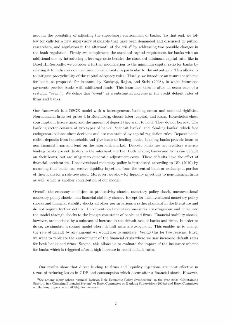
Our results show that direct lending to firms and liquidity injections are most effective in

terms of reducing losses in GDP and consumption which occur after a financial shock. However,

2See among many others “Annual Jackson Hole Economic Policy Symposium” in the year 2008 “MaintainingStability in a Changing Financial System” or Basel Committee on Banking Supervision (2009a) and Basel Committeeon Banking Supervision (2009b), for instance.

2

when we take volatilities into account, direct lending to firms leads to the highest fluctuation

in inflation and second highest volatility in GDP. Liquidity injections also strongly increase the

volatility of GDP and inflation. Asset swaps, on the contrary, have almost no impact, neither on

GDP and consumption losses, nor on the volatility of inflation, GDP, and consumption. Stricter

bank regulatory requirements reduce losses in GDP with almost no impact on volatilities. When

unconventional monetary policy is combined with stricter bank regulation, we find that qualitative

easing becomes more effective in terms of reducing losses in GDP and consumption, whereas

quantitative easing becomes less effective. Interestingly, direct lending to firms becomes even

more effective in mitigating losses in GDP and consumption when combined with a leverage ratio

requirement like in Basel III.

The rest of this paper is organized as follows. The setup of the basic model is introduced in

Section 1.2. In Section 1.3, we discuss the calibration of the model. Section 1.4, we conduct the

impulse response analysis and discuss results. Section 1.5 concludes.

2 The Baseline Model

Our framework is a DSGE model with nominal rigidities. The economy is inhabited by households,

banks, non-financial firms, and a central bank. Banking sector consists of deposit and lending banks

which interact in an interbank market. Central bank conducts both conventional and unconven-

tional monetary policy; as our model lacks any distinct fiscal or supervisory authorities, we assume

that the central bank takes over those roles. In particular, it supervises banking sector through

capital and leverage ratios.

Overall, the economy is subject to various perturbations: productivity, monetary policy, quan-

titative, and qualitative monetary easing shocks to banks and firms as well as financial stability

shocks.

2.1 Households

Households allocate their resources to consumption Ct and investments and choose their leisure

time (1−Nt). They provide labor Nt against wage wt, place deposits Dht against an interest rate

rlt with deposit banks and do not borrow. Following de Walque et al. (2009) we impose a target

in deposits Dh via a quadratic disutility term3. This means that households dislike deviations of

their deposits from the long-run optimal level. The households maximization program is given by:

maxCt,Nt,D

ht

∞∑

s=0

βsEt

log (Ct+s) +m log (1−Nt+s)−χ

2

(

Dht

1 + rlt+s

−

Dh

1 + rl

)2

(1)

under the budget constraint:

Ct +Dh

t

1 + rlt= wtNt +

Dht−1

πt+Πf

t + (1− vb)Πbt + (1− vl)Π

lt (2)

where πt = Pt/Pt−1 is inflation and Πft , Π

bt , Π

lt are profits of firms, lending banks, and deposit

3This term is necessary for technical reasons. For χ = 0, first order conditions in (29) and (36) give the steadystate for rlt leaving Dh

t undetermined. χ is kept very low so that the dynamics of the model are not alteredsignificantly by its use.

3

banks, respectively. Households fully own firms and they receive a share of banks profits in line

with retained earnings ratios vb and vl.

First order conditions of the households optimization problem are presented in the Appendix.

2.2 Non-financial Firms

Entrepreneurs choose price P (i)t, labor N (i)t, capital K (i)t, loans L (i)ft to rebuild capital stock

and repayment rate on past borrowings α (i)t from the profit maximization. They face price

adjustment costs a la Rotemberg which introduce a nominal rigidity into the model.

maxP (i)

t,K(i)

t,N(i)

t,L(i)ft ,α(i)t

∞∑

s=0

Etβt+sΠ(i)ft+s (3)

where the profit is given by:

Π (i)ft =

P (i)tPt

Y (i)t − wtN (i)t −α (i)t L (i)

ft−1

πt−

M (i)ft−1

πt

−

γ

2

[

(

1− α (i)t−1

)

(

L (i)ft−2

πt−1+ df

)]2

−

ψ

2

(

P (i)tP (i)t−1

− π∗

)2

Yt (4)

π∗ is the economy-wide inflation rate and the parameter ψ measures the degree of price sticki-

ness. The higher ψ, the more sluggish is the adjustment of nominal prices; ψ = 0 implies flexible

prices. In addition, non-financial firms bear quadratic costs of default on their loans4. At times of

financial distress, when bank lending is scarce or difficult to obtain, central bank may step in and

provide firms with additional liquidity M (i)ft in order to help them to build up capital needed for

production.

The production sector comprises of a continuum of monopolistically competitive firms each

facing a downward-sloping demand curve for its differentiated product

Y (i)t =

(

P (i)tPt

)

−θ

Yt (5)

where P (i)t is the profit-maximizing price consistent with production level Y (i)t. Parameter θ

is the elasticity of substitution between two differentiated goods. Both the aggregate price level Pt

and aggregate output Yt are beyond control of the individual firm. The aggregates for the economy

are written as

Yt = Kηt (exp (At)Nt)

1−η (6)

4The expenses related to default consist of a variable part that relates to the notional of outstanding loans in

the economy,(

1− α (i)t−1

)

L(i)ft−2

πt−1, and an additional fixed cost,

(

1− α (i)t−1

)

df . Linearity of cost would imply

indeterminacy for (32); partition of cost is done in analogy to the setup of the maximization problem for lendingbanks, where this partitioning allows to reconcile (36), (39) and (41) when determining steady state values for rbt ,rlt and it.

de Walque et al. (2009) solve this technicality by splitting the expenses related to default into non-pecuniarycosts that affect utility and pecuniary costs that impact profits. However, as they acknowledge, this ’double cost’lacks pure micro foundations. In our opinion, segmentation of the pecuniary default costs into a fixed and variableportion is more appealing micro-economically.

4

Kt = (1− τ)Kt−1 +Lft

1 + rbt+

Mft

1 + rt(7)

At = ρaAt−1 + εAt (8)

where firms produce output according to a Cobb-Douglas function with At functioning as

an aggregate productivity shock. Equation (7) describes the law of motion for capital which

depreciates at rate τ . Firms can obtain loans from lending banks Lft at interest rate rbt or receive

liquidity from the central bank Mft at times of financial distress. Since firms are fully owned by

households, their discount factor is given by:

βt+s = βs Ct

Ct+s

(9)

First order conditions are solved assuming a symmetric equilibrium and are presented in the

Appendix.

2.3 Banks

When modeling the banking sector we lean on de Walque et al. (2009) and Dib (2010) and introduce

deposit banks and lending banks. Both types of banks are risk-averse.

Deposit Banks

Deposit banks collect deposits from households Dlt and provide lending banks with loans Dbs

t on

the interbank market. They also allocate their resources to a market book Bl, which is assumed to

be exogenous and to yield a return ρ. In addition, deposit banks derive utility from holding own

funds F lt above the capital requirement k and the leverage limit h - both imposed by the central

bank - but they face opportunity costs rtFlt of maintaining these funds. We define leverage ratio

as an inverse of the leverage multiple which is a ratio of total assets to equity. Contrary to the

capital ratio, leverage ratio does not involve any riskiness weights of the assets and it serves as a

primal measure of the sheer size of the balance sheet. In our basic setup we first assume that the

central bank does not care about leverage ratio (bF l = 0); then, in Section 4, we present simulation

results for the case when leverage ratio does become an instrument of financial regulation.

The maximization program of the deposit banks is:

maxDl

t,Dbst

∞∑

s=0

Etβt+s

log(

Πlt+s

)

+ dF l

[

F lt+s − k

(

wl(

Dbst+s − xlt+s

)

+ wBl)]

+bF l

[

F lt+s − h

(

Dbst+s +B

l)]

(10)

under the constraints:

Πlt =

δtDbst−1

πt−

Dbst

1 + rit+

Dlt

1 + rlt−

Dlt−1

πt+ ζl (1− δt−1)

Dbst−2

πt−1+ρB

l

πt

+xlt −xlt

1 + rt+

M lt

1 + rt−

M lt−1

πt− rtF

lt (11)

5

F lt = (1− ξl +l)

F lt−1

πt+ vlΠ

lt (12)

Loans on the interbank market are prone to lending banks’ default rate (1− δt). Deposit banks’

own funds increase by a share of profits that are not redistributed to households vlΠlt; a small pro-

portion of funds ξl is put into an insurance scheme run by the central bank. A fraction ζl of the

lending banks’ defaulted amount is paid back from this insurance, decreasing the losses suffered

from impaired loans on the interbank market. Another portion of the insurance payout, provided

by the central bank, is aimed to increase equity of the deposit banks by l. This insurance payout

kicks in only if the solvency of the lending banks deteriorates notably.

Furthermore, deposit banks can exchange a portion of their lending for a risk-free asset xlt as

a measure of so called qualitative easing policy conducted by the central bank. The quantitative

policy actions, i.e. liquidity injections, operate through M lt . We assume that the portion of assets

xlt under the swap agreement is impaired and would not pay any return otherwise.

First order conditions are presented in Appendix.

Lending Banks

Equivalently to deposit banks, lending banks derive additional utility from holding extra funds F bt

(above the levels implied by the capital and leverage ratios) at the opportunity cost of rtFbt . The

maximization program of lending banks is given by:

maxDbd

t ,Lbt ,δt

∞∑

s=0

Etβt+s

log(

Πbt+s

)

+ dF b

[

F bt+s − k

(

wb(

Lbt+s − xbt+s

)

+ wBb)]

+bF b

[

F bt+s − h

(

Lbt+s +B

b)]

(13)

under the constraints:

Πbt =

αtLbt−1

πt−

Lbt

1 + rbt+

Dbdt

1 + it−

δtDbdt−1

πt−

ω

2

[

(1− δt−1)

(

Dbdt−2

πt−1+ dδ

)]2

+ζb (1− αt−1)Lbt−2

πt−1+ρB

b

πt+ xbt −

xbt1 + rt

+M b

t

1 + rt−

M bt−1

πt− rtF

bt (14)

F bt = (1− ξb +b)

F bt−1

πt+ vbΠ

bt (15)

Lending banks provide loans to the firms Lbt , borrow from deposit banks Dbd

t , invest in an

exogenous market book Bbat yield of ρ, and choose their optimal repayment rate δt. In addition,

lending banks can receive liquidity injections from the central bank M bt (quantitative easing) or

swap a fraction of their loans against a risk-free asset xbt (qualitative easing). We assume that

xbt is impaired in that it pays no return when retained in the loan portfolio. Lending banks face

pecuniary costs of default represented by a quadratic cost function ω2

[

(1− δt−1)(

Dbdt−2

πt−1+ dδ

)]2

.

Quadratic formulation prevents indeterminacy in the first order condition (41); dδ stands for a

fixed costs of default which are independent from the total amount of the defaulted interbank

loans (1− δt−1)Dbd

t−2

πt−1.

6

Similar to deposit banks, lending banks increase own funds by a share of profits that are not

redistributed to households vbΠbt ; a small proportion of funds ξb is put into an insurance scheme,

which is motivated by the fact that lending banks face losses on their loans to firms in accordance

with firms’ defaults ratio (1− αt). A fraction ζb of the firms’ defaulted amount is reimbursed by

the insurance. In the case of a substantial increase in firms default rate, lending banks may be

supported by equity capital b provided by the central bank.

First order conditions are presented in the Appendix.

2.4 Central Bank

The monetary authority conducts its policy according to a Taylor-type policy rule:

(1 + rt) = (1 + r)(1−µr) (1 + rt−1)

µr

( πtπ∗

)Qp

(

YtYt−1

)Qy

exp (εrt ) (16)

At times of financial distress it can use unconventional instruments: liquidity injections M(·)t

(quantitative easing) or qualitative monetary easing x(·)t aimed at supporting both types of banks

and firms. We model all unconventional monetary tools as AR (1) processes:

xlt = ρxxlt−1 + εx

l

t (17)

xbt = ρxxbt−1 + εx

b

t (18)

M lt = ρMM

lt−1 + εM

l

t (19)

M bt = ρMM

bt−1 + εM

b

t (20)

Mft = ρMM

ft−1 + εM

f

t (21)

It is assumed that the deposit, interbank, and commercial loan markets clear in the long run.

However, in the short run the central bank may inject liquidity such that:

M lt = Dl

t −Dht (22)

M bt = Dbs

t −Dbdt (23)

Mft = Lf

t − Lbt (24)

By assumption, the central bank finances liquidity injections, capital injections to banks, asset

swaps, and payoffs from the insurance scheme by collecting contributions from banks.

7

3 Calibration

In the calibration we push our model towards a steady state with very low interest rates (around

0.5%) and yields on the market book (1%) in order to simulate an environment of low asset returns.

Real sector

We normalize employment to 0.2 and use Cobb-Douglas production function with labor share

= 2/3. We utilize the assumption that capital stock is 10 times higher than production and set

depreciation rate at 3%. This implies an investment ratio to output of 0.3 and allows us to avoid

a negative search cost γ on the defaulted amount. ρa, the autoregression coefficient for the tech-

nology equation (8), is equal 0.95 which is a standard in the RBC literature.

We set the value for the default rate of firms equal to 5% (an therefore αt = 0.95 in steady

state) which is inferred from the US courts and the Bureau of Labor Statistics quarterly pre-crisis

data on business bankruptcies. The data are based on the number of non-financial corporations

that go bankrupt. This enables us to deduct values for γ (firms default cost parameter) and m

(households leisure utility parameter). Both firms fixed default cost parameter and the smoothing

parameter for deposits are set close to 0 (χ = 0.01, df = 0.001), in order to eschew any dynamic

effects (positive χ enforces finding a steady state value for Dht ). We also introduce a penalty pa-

rameter for setting prices above the economy-wide level of 50, which we obtain by comparing the

elasticity of inflation to the real marginal cost in our model with the slope coefficient of the log-

linear Phillips curve using a Calvo approach. Expressed as (1−δ)(1−βδ)δ

, where δ is the probability

of not resetting the price, this slope coefficient is found in the literature to be around 0.75 (see

discussion of the frequency of price adjustment in Faia and Monacelli (2007), for instance).

Banking sector

In order to simulate the environment of low interest rates we set the deposit rate at rl= 0.35%

and assume that the market book offers a mere ρ = 1%, which lies below the average quarterly

return of the Dow Jones Industrial Average Index from 1980Q1 to 2010Q3 (1.96%). However, this

assumption may actually be somehow questionable due to possible assets bubbles when interest

rates, i.e. borrowing costs are extremely low.

We set lending banks default rate δ = 0.98 which is derived from the pre-crisis data provided by the

Federal Deposit Insurance Corporation. These data encompasses the number of bank failures. Fur-

thermore, when calibrating the model we impose Dl/Lb to be around 2, Dbd/Lb = Dbs/Lbaround

0.5, which is in line with pre-crisis statistics of the Federal Reserve System. The market book for

each bank equals firm loans: Bb= B

l= Lb.

The weights of bank assets are aligned to the Basel agreement: wb = 0.8 and wl = 0.05. Capital

ratio is set at k = 8% and leverage ratio at h = 4%. Banks are supposed to allocate half of their

profits to own funds (vb = vl = 0.5) and the remaining 50% are distributed to the households.

The insurance scheme is assumed to enable banks to recover 80% of bad loans; in exchange, banks

must pay premia of around 6 − 7% of their funds (ξb = 0.06 and ξl = 0.07, due to differences in

default rates for firms and lending banks) in order to benefit from this provision. The parameter

8

of fixed default costs for lending banks dδ is equal to 0.001.

Other parameters - default cost parameter ω and own funds utility parameters for both bank

types, dF b , dF l , bF b and bF l - are inferred from the restrictions mentioned above.

Central bank

Taylor-type monetary policy rule contains parameters that are set according to specifications used

in the literature and satisfy the Taylor rule principle (µr = 0.7, Qp = 1.2, Qy = 0.05). Regression

parameters for all unconventional monetary tools (ρ(·)) are set to 0.85.

4 Quantitative Results

4.1 Impulse Responses

In this section we examine dynamic properties of our model by means of impulse response analy-

sis. We investigate how shocks propagate through the system and affect the key macroeconomic

variables. Our analysis starts with a short review of impulse responses to innovations in technol-

ogy and monetary policy and then it passes on to inspection of shocks induced by unconventional

monetary policy actions.

Standard analysis: Technology and monetary policy shocks

Figure 5 in the Appendix shows that a positive technology shock has positive effects on consump-

tion, capital, output, and GDP. In the short run all interest rates and inflation increase, but after

about 10 periods they all fall below their initial steady state levels. Interbank, deposit, and firms’

lending rates react in a less pronounced way than the policy rate due to the adjustment costs of

changing those rates.

Following the positive technology shock, demand for capital increases and is matched by a ris-

ing supply of loans to the firms. On the impact of the shock, profits of banks grow; however, firms’

profits initially decline before returning to their pre-shock steady state level. This is due to rising

capital costs caused by more expensive loans which also drives up the marginal cost. On the one

hand, increases in the borrowing rate for capital reduces firms’ profits. On the other hand, firms

are subject to constraints set by price adjustment cost when trying to pass on the loan burden to

consumers. Finally, positive technology shock leads to falling default rates for firms and lending

banks; interest rates and inflation decrease in the long-run as a result of higher productivity and

output.

When compared to Dib (2010) we observe responses to the technology shock in our model to

be generally in line with his results. Notable exceptions are inflation and the policy rate where

slightly different patterns of reaction can be observed. Dib (2010) finds that both fall immediately

after the shock occurs and return gradually to their initial steady state levels thereafter. Yet, it

seems to be reasonable that after a positive technology shock interest rates should increase. Two

arguments speak in favor for this notion. First, central bank would increase its policy rate to close

the output gap; second, higher demand for firm loans leads to an increase in interbank borrowing

9

and thus to a rising demand for deposits. Consequently, the interest rates for these aggregates

should increase.

As shown in Figure 6 in the Appendix, an expansionary monetary policy shock produces per-

sistent moves in inflation and interest rates (except for the policy rate itself whose shock we model

as an AR(1) process). After the monetary policy shock, consumption and capital increase; output

stays almost unchanged; GDP grows, however, the effect on it seems to fade away relatively quickly.

After the expansionary monetary policy shock banks’ profits expand; in case of lending banks, this

is due to rising demand for commercial loans and improving solvency within firms. In the case

of deposit banks, this is causes by the fact that the interest rate for their liabilities is decreasing

stronger than the interest rate for their assets. Reaction of inflation is somehow puzzling as we

would expect it to rise after a decrease in the policy rate. This is presumably attributable to the

model setup in which production sector simultaneously marks up its production. Falling interest

rates throughout the economy contribute to the reduction in marginal cost for firms, i.e. reduction

in capital costs weights out rising labor cost. However, firms’ profits tend to decrease temporarily

on the impact of the monetary policy shock as initially the build-up in capital is not matched by

an increase in output.

Dib’s (2010) analysis points to decreasing industrial loans and a short-run increase in the firms’

borrowing rate after the expansionary monetary policy rate shock hits the economy. In our model,

however, this shock leads to a fall in the borrowing rate along with an increased demand for firms’

loans. We interpret our result as more intuitive since it reconfirms the expectation of falling interest

rates throughout the whole economy after a cut in the policy rate.

Unconventional monetary policy

Figure 1 displays impulse responses after a liquidity injection to lending banks. This shock tends

to have only temporary effects on economic aggregates. It decreases the risk-free rate, inflation,

firms’ borrowing rate, deposit rate, and the interbank interest rate. Figure 1 shows that following

a liquidity shock, output, and GDP rise, yet their reaction - like for most of the variables - is not

persistent. This effect is due to the persistence of liquidity itself as it is an AR(1) process with lag

parameter ρMb . Since we assume that in the steady state the interbank market clears, liquidity

injections are equal to zero in the long run. Imbalances in the interbank market after the liquidity

shock are then quickly forced to equilibrium by the movement in the interbank interest rate and an

adjustment in default rate of lending banks. Liquidity injection to lending banks seems to crowd

out interbank loans and improve lending bank profits as they choose to default on a portion of

their interbank borrowing given cheaper refinancing from the central bank. Deposit bank profits

improve as well due to falling deposit rates.

Our results generally reconfirm the findings of Dib (2010). Output, consumption, inflation,

policy rate, and other aggregates show the same pattern of behavior after the shock, however, they

differ in persistence.

Liquidity injections to deposit banks serve as an instrument of supporting interbank market by

strengthening the liquidity position of deposit banks (for instance, in case of significant deposit

withdrawals). As shown in Figure 7 in the Appendix such liquidity injections to deposit banks

10

Figure 1: Figure 1.1: Impulse responses after a liquidity injection shock to lending banks

5 10 15 20 25 30−0.1

−0.05

0interbank rate

5 10 15 20 25 30−0.1

−0.05

0firms borrowing rate

5 10 15 20 25 30−0.1

−0.05

0deposit rate

5 10 15 20 25 30−0.2

−0.1

0risk−free rate

5 10 15 20 25 30−0.1

−0.05

0inflation

5 10 15 20 25 30−10

0

10loans to firms supply

5 10 15 20 25 30−10

0

10loans to firms demand

5 10 15 20 25 30−20

0

20loans to lending banks supply

5 10 15 20 25 30−20

0

20loans to lending banks demand

5 10 15 20 25 30−5

0

5deposit supply

5 10 15 20 25 30−5

0

5deposit demand

5 10 15 20 25 300

0.5

1lending banks capital

5 10 15 20 25 300

0.5deposit banks capital

5 10 15 20 25 30−0.05

0

0.05consumption

5 10 15 20 25 300

0.2

0.4capital

5 10 15 20 25 300

0.1

0.2output

5 10 15 20 25 300

0.02

0.04wage

5 10 15 20 25 30−2

−1

0marginal cost

5 10 15 20 25 30−100

0

100firms profits

5 10 15 20 25 30−1

0

1lending banks profits

5 10 15 20 25 30−1

0

1deposit banks profits

5 10 15 20 25 30−5

0

5GDP

5 10 15 20 25 30−0.5

0

0.5solvency − firms

5 10 15 20 25 30−0.2

0

0.2solvency − lend. banks

generate responses that are quite similar to those following a quantitative monetary easing shock

to lending banks. Yet its impact on GDP, consumption, and in part on output tends to be of

limited duration. Notable is also a non-negative effect on lending banks default rate. Even though

M lt is injected at rt > rlt and thus above the initial refinancing cost, deposit bank profits rise and

so does their capital, which by definition is partly cumulated from retained earnings. Lowering the

price of this liquidity injection even further would, of course, have a positive influence on deposit

bank profits, leaving its impact on other aggregates unchanged.

Figure 2: Figure 1.2: Impulse responses after a liquidity injection shock to firms

5 10 15 20 25 30−0.05

0

0.05interbank rate

5 10 15 20 25 30−0.1

0

0.1firms borrowing rate

5 10 15 20 25 30−0.05

0

0.05deposit rate

5 10 15 20 25 30−0.2

0

0.2risk−free rate

5 10 15 20 25 30−0.1

0

0.1inflation

5 10 15 20 25 30−10

0


5 10 15 20 25 30−5

0


5 10 15 20 25 30−20

0


5 10 15 20 25 30−20

0


5 10 15 20 25 30−5

0

5deposit supply

5 10 15 20 25 30−5

0

5deposit demand

5 10 15 20 25 30−0.5

0

0.5lending banks capital

5 10 15 20 25 30−0.5

0


5 10 15 20 25 30−0.05

0

0.05consumption

5 10 15 20 25 300

0.2

0.4capital

5 10 15 20 25 30−0.2

0

0.2output

5 10 15 20 25 300

0.02

0.04wage

5 10 15 20 25 30−2

0

2marginal cost

5 10 15 20 25 30−100

0

100firms profits

5 10 15 20 25 30−1

0


5 10 15 20 25 30−0.5

0

0.5deposit banks profits

5 10 15 20 25 30−5

0

5GDP

5 10 15 20 25 30−0.2

0


5 10 15 20 25 30−0.5

0


As illustrated in Figure 2, liquidity supply directed at firms improves output but has only a

11

limited impact on GDP and consumption. When the central bank lends directly to firms, this

action tends to crowd out bank loans to firms and to decrease lending on the interbank market.

Motivated by cheaper financing, firms decide to default on some of its bank loans which in turn

forces some of the lending banks to dishonor their debt. Altogether, impact to GDP is almost nil;

only capital Kt and lending banks capital F bt increase but all other components fall.

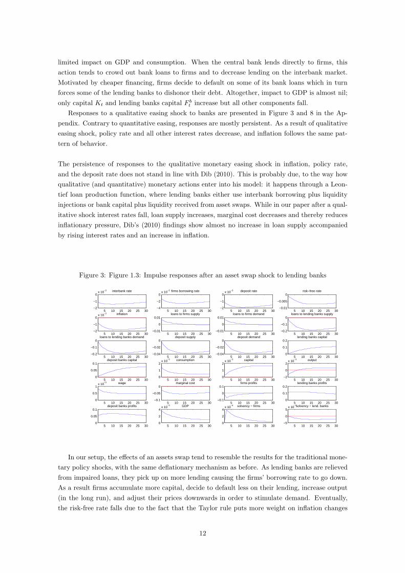
Responses to a qualitative easing shock to banks are presented in Figure 3 and 8 in the Ap-

pendix. Contrary to quantitative easing, responses are mostly persistent. As a result of qualitative

easing shock, policy rate and all other interest rates decrease, and inflation follows the same pat-

tern of behavior.

The persistence of responses to the qualitative monetary easing shock in inflation, policy rate,

and the deposit rate does not stand in line with Dib (2010). This is probably due, to the way how

qualitative (and quantitative) monetary actions enter into his model: it happens through a Leon-

tief loan production function, where lending banks either use interbank borrowing plus liquidity

injections or bank capital plus liquidity received from asset swaps. While in our paper after a qual-

itative shock interest rates fall, loan supply increases, marginal cost decreases and thereby reduces

inflationary pressure, Dib’s (2010) findings show almost no increase in loan supply accompanied

by rising interest rates and an increase in inflation.

Figure 3: Figure 1.3: Impulse responses after an asset swap shock to lending banks

5 10 15 20 25 30−2

−1

0x 10

−3 interbank rate

5 10 15 20 25 30−4

−2

0x 10

−3 firms borrowing rate

5 10 15 20 25 30−2

−1

0x 10

−3 deposit rate

5 10 15 20 25 30−0.01

−0.005

0risk−free rate

5 10 15 20 25 30−2

−1

0x 10

−3 inflation

5 10 15 20 25 30−0.01

0

0.01loans to firms supply

5 10 15 20 25 30−0.01

0

0.01loans to firms demand

5 10 15 20 25 30−0.2

−0.1


5 10 15 20 25 30−0.2

−0.1


5 10 15 20 25 30−0.04

−0.02

0deposit supply

5 10 15 20 25 30−0.04

−0.02

0deposit demand

5 10 15 20 25 300

0.1


5 10 15 20 25 300

0.05


5 10 15 20 25 300

1

2x 10

−3 consumption

5 10 15 20 25 300

1

2x 10

−3 capital

5 10 15 20 25 30−2

0

2x 10

−3 output

5 10 15 20 25 300

0.5

1x 10

−3 wage

5 10 15 20 25 30−0.1

−0.05

0marginal cost

5 10 15 20 25 30−0.1

0

0.1firms profits

5 10 15 20 25 300

0.1

0.2lending banks profits

5 10 15 20 25 300

0.05


5 10 15 20 25 300

2

4x 10

−3 GDP

5 10 15 20 25 300

2

4x 10

−4 solvency − firms

5 10 15 20 25 30−5

0

5x 10

−3solvency − lend. banks

In our setup, the effects of an assets swap tend to resemble the results for the traditional mone-

tary policy shocks, with the same deflationary mechanism as before. As lending banks are relieved

from impaired loans, they pick up on more lending causing the firms’ borrowing rate to go down.

As a result firms accumulate more capital, decide to default less on their lending, increase output

(in the long run), and adjust their prices downwards in order to stimulate demand. Eventually,

the risk-free rate falls due to the fact that the Taylor rule puts more weight on inflation changes

12

than on the output fluctuations.

All variables, except for loans to lending banks, react similarly to the quantitative easing aimed

at deposit banks as they did in case of this type of central bank action addressed at the lending

banks (see Figure 8 in the Appendix). The possibility for deposit banks to swap their interbank

loans has the same impact on the balance sheet of deposit bank as swaps of firm loans have on the

balance sheet of lending banks: when the central bank absorbs impaired loans from banks’ balance

sheet (and thus improves deposit banks capital ratio), they instantly expand their lending on the

interbank market at a lower price which, in turn, enhances solvency of lending banks.

When we compare the impulse responses for both types of banks, we observe that the solvency

of firms, in both cases, increases remarkably in the short run and remains above its steady state

in the medium to long run. However, the solvency of lending banks is decreasing when lending

banks are allowed to swap their assets, but is strongly increasing in the short run and it remains

above its steady state over the long horizon when deposit banks are the profiteers of the qualitative

easing. This result indicates that qualitative monetary easing measures aimed at deposit banks

can improve the stability of the financial system.

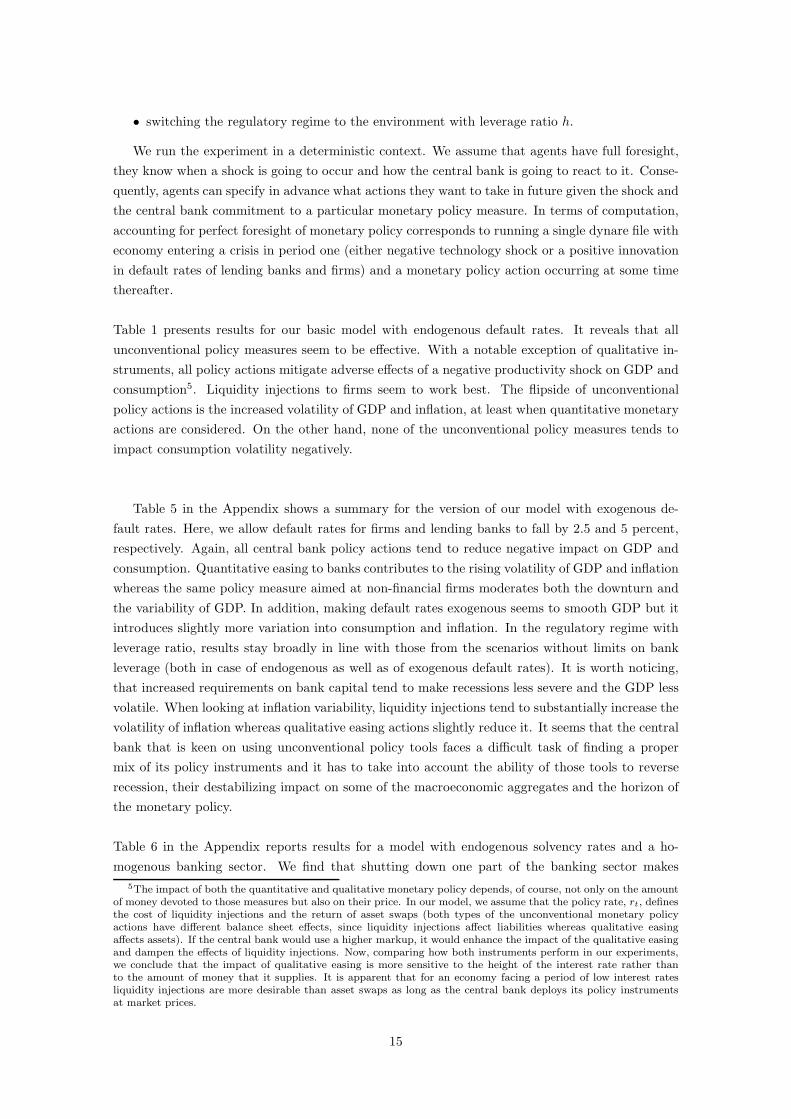
As Figure 4 shows, insurance payout to lending banks’ improves their solvency and has a per-

sistent effect on the economy. It also increases loans to firms, raises their production capital

marginally and that in turn leads to a raise in output. Since the Taylor rule is driven by output

and inflation, the growth of output results in an increase of the policy rate. The subsequent rising

in interest rates have an ambiguous impact on economy: they increase the marginal cost of capital

for firms which are now trying to substitute capital with labor; in addition, higher interest rates

make consumption less desirable and therefore push households towards more labor supply result-

ing in lower wages. As marginal cost increases, firms mark up the prices letting policy interest

rate to climb up even further. As commercial loan costs pick up, firms choose to default on some

of their debt. Deposit and lending banks profits fall since in steady state their liabilities (deposits

and interbank loans) outweigh their assets (interbank loans and loans to firms) in absolute terms,

which leads to losses in the case of rising interest rates.

We observe in Figure 9 in the Appendix that a similar mechanism is at work in case of an

increase in deposit banks’ equity. Generally, the responses tend towards rising interest rates,

inflation and marginal cost of production whereas consumption, wage, and production capital tend

to fall. However, after an initial pick-up in credit supply to the economy, loans tend to fall in both

real and financial sectors and as the level of interest rates raises, both firms and lending banks

choose to default on more of their debt. The marginal increase in GDP seems to result from a

small rise in the deposit banks’ capital, as other components of GDP tend to fall.

4.2 Experiments

In this section we intend to simulate crisis conditions and then consider the role of central bank’s

instruments of unconventional monetary policy in moderating the crisis. We conduct experiments

with two versions of our model: the basic one, where default rates are endogenously chosen by

13

Figure 4: Figure 1.4: Impulse responses after a capital injection shock to lending banks

5 10 15 20 25 300

0.5

1x 10

−3 interbank rate

5 10 15 20 25 300

1

2x 10


5 10 15 20 25 300

1

2x 10

−3 deposit rate

5 10 15 20 25 300

5x 10

−3 risk−free rate

5 10 15 20 25 300

1

2x 10

−3 inflation

5 10 15 20 25 300

1

2x 10

−3 loans to firms supply

5 10 15 20 25 300

1

2x 10

−3loans to firms demand

5 10 15 20 25 300

0.1

0.2loans to lending banks supply

5 10 15 20 25 300

0.1

0.2loans to lending banks demand

5 10 15 20 25 300

0.02

0.04deposit supply

5 10 15 20 25 300

0.02

0.04deposit demand

5 10 15 20 25 300

2


5 10 15 20 25 30−0.1

−0.05

0deposit banks capital

5 10 15 20 25 30−1

−0.5

0x 10

−3 consumption

5 10 15 20 25 30−1

0

1x 10

−3 capital

5 10 15 20 25 30−1

0

1x 10

−3 output

5 10 15 20 25 30−4

−2

0x 10

−4 wage

5 10 15 20 25 300

0.02

0.04marginal cost

5 10 15 20 25 30−0.01

0

0.01firms profits

5 10 15 20 25 30−0.5

0


5 10 15 20 25 30

−0.04

−0.02


5 10 15 20 25 30−0.05

0

0.05GDP

5 10 15 20 25 30−2

0

2x 10


5 10 15 20 25 30−2

0

2x 10


firms and lending banks and another version in which default rates are exogenously given as AR (1)

processes:

αt = ρααt−1 + εαt (25)

δt = ρδδt−1 + εδt (26)

The timeline looks as follows: in the 1st period a shock that introduces a downturn of the

economy occurs. In the first scenario it is a two standard deviations negative productivity shock;

in the second version of the model with exogenous default rates we let the firms’ and lending banks’

solvency ratios fall by 2.5% and 5% respectively. This is supposed to replicate the origin of the

ongoing financial crisis. In the 2nd period the central bank steps in with its unconventional policy

actions. We assume that in each case it commits 5% of GDP into its unconventional policy tools.

We then evaluate the welfare effects simply by comparing present values of future consumption

and GDP once central bank anti-crisis actions have been put in place. In particular, we take into

account:

• liquidity injections to banks and firms,

• asset swaps to banks,

• switching the regulatory regime to the environment where capital ratio k is a function of

output gap such that:

(1 + kt) = (1 + k)

(

YtYt−1

)Qk

exp(

εkt)

(27)

• direct capital injections to lending and deposit banks,

14

• switching the regulatory regime to the environment with leverage ratio h.

We run the experiment in a deterministic context. We assume that agents have full foresight,

they know when a shock is going to occur and how the central bank is going to react to it. Conse-

quently, agents can specify in advance what actions they want to take in future given the shock and

the central bank commitment to a particular monetary policy measure. In terms of computation,

accounting for perfect foresight of monetary policy corresponds to running a single dynare file with

economy entering a crisis in period one (either negative technology shock or a positive innovation

in default rates of lending banks and firms) and a monetary policy action occurring at some time

thereafter.

Table 1 presents results for our basic model with endogenous default rates. It reveals that all

unconventional policy measures seem to be effective. With a notable exception of qualitative in-

struments, all policy actions mitigate adverse effects of a negative productivity shock on GDP and

consumption5. Liquidity injections to firms seem to work best. The flipside of unconventional

policy actions is the increased volatility of GDP and inflation, at least when quantitative monetary

actions are considered. On the other hand, none of the unconventional policy measures tends to

impact consumption volatility negatively.

Table 5 in the Appendix shows a summary for the version of our model with exogenous de-

fault rates. Here, we allow default rates for firms and lending banks to fall by 2.5 and 5 percent,

respectively. Again, all central bank policy actions tend to reduce negative impact on GDP and

consumption. Quantitative easing to banks contributes to the rising volatility of GDP and inflation

whereas the same policy measure aimed at non-financial firms moderates both the downturn and

the variability of GDP. In addition, making default rates exogenous seems to smooth GDP but it

introduces slightly more variation into consumption and inflation. In the regulatory regime with

leverage ratio, results stay broadly in line with those from the scenarios without limits on bank

leverage (both in case of endogenous as well as of exogenous default rates). It is worth noticing,

that increased requirements on bank capital tend to make recessions less severe and the GDP less

volatile. When looking at inflation variability, liquidity injections tend to substantially increase the

volatility of inflation whereas qualitative easing actions slightly reduce it. It seems that the central

bank that is keen on using unconventional policy tools faces a difficult task of finding a proper

mix of its policy instruments and it has to take into account the ability of those tools to reverse

recession, their destabilizing impact on some of the macroeconomic aggregates and the horizon of

the monetary policy.

Table 6 in the Appendix reports results for a model with endogenous solvency rates and a ho-

mogenous banking sector. We find that shutting down one part of the banking sector makes

5The impact of both the quantitative and qualitative monetary policy depends, of course, not only on the amountof money devoted to those measures but also on their price. In our model, we assume that the policy rate, rt, definesthe cost of liquidity injections and the return of asset swaps (both types of the unconventional monetary policyactions have different balance sheet effects, since liquidity injections affect liabilities whereas qualitative easingaffects assets). If the central bank would use a higher markup, it would enhance the impact of the qualitative easingand dampen the effects of liquidity injections. Now, comparing how both instruments perform in our experiments,we conclude that the impact of qualitative easing is more sensitive to the height of the interest rate rather thanto the amount of money that it supplies. It is apparent that for an economy facing a period of low interest ratesliquidity injections are more desirable than asset swaps as long as the central bank deploys its policy instrumentsat market prices.

15

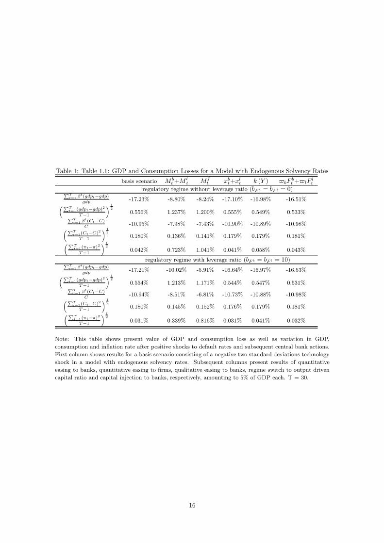
Table 1: Table 1.1: GDP and Consumption Losses for a Model with Endogenous Solvency Rates

basis scenario M bt+M

lt Mf

t xbt+xlt k (Y ) bF

bt +lF

lt

regulatory regime without leverage ratio (bF b = bF l = 0)∑T

t=1 βt(gdpt−gdp)

gdp-17.23% -8.80% -8.24% -17.10% -16.98% -16.51%

(∑Tt=1(gdpt−gdp)2

T−1

)12

0.556% 1.237% 1.200% 0.555% 0.549% 0.533%∑T

t=1 βt(Ct−C)

C-10.95% -7.98% -7.43% -10.90% -10.89% -10.98%

(∑Tt=1(Ct−C)2

T−1

)12

0.180% 0.136% 0.141% 0.179% 0.179% 0.181%(∑

Tt=1(πt−π)2

T−1

)12

0.042% 0.723% 1.041% 0.041% 0.058% 0.043%

regulatory regime with leverage ratio (bF b = bF l = 10)∑

Tt=1 βt(gdpt−gdp)

gdp-17.21% -10.02% -5.91% -16.64% -16.97% -16.53%


T−1

)12

0.554% 1.213% 1.171% 0.544% 0.547% 0.531%∑

Tt=1 βt(Ct−C)

C-10.94% -8.51% -6.81% -10.73% -10.88% -10.98%

(∑Tt=1(Ct−C)2

T−1

)12

0.180% 0.145% 0.152% 0.176% 0.179% 0.181%(∑

Tt=1(πt−π)2

T−1

)12

0.031% 0.339% 0.816% 0.031% 0.041% 0.032%

Note: This table shows present value of GDP and consumption loss as well as variation in GDP,

consumption and inflation rate after positive shocks to default rates and subsequent central bank actions.

First column shows results for a basis scenario consisting of a negative two standard deviations technology

shock in a model with endogenous solvency rates. Subsequent columns present results of quantitative

easing to banks, quantitative easing to firms, qualitative easing to banks, regime switch to output driven

capital ratio and capital injection to banks, respectively, amounting to 5% of GDP each. T = 30.

16

recessions more severe in terms of GDP and consumption loss. Standard deviation of GDP and

consumption rises whereas the variability of inflation decreases slightly. We conclude that having

a heterogeneous banking sector enhances economy’s resilience against economic downturns and

moderates the variation in the most macroeconomic aggregates. In addition, the heterogeneity of

banks also improves the effects of monetary policy actions.

Generally, results from Tables 1 and 5 suggest, that a central bank which puts more weight on tar-

geting inflation should use more qualitative easing tools. On the other hand, a central bank which

primarily focuses on GDP should apply quantitative easing instruments. Therefore, the inflation

targeting central bank would observe a higher output gap when trying to manage inflation in the

short run whereas central bank that stabilizes GDP in the long run would produce an excessive

inflation variability6.

5 Conclusion

The ongoing financial crisis revealed that standard DSGE models need to account for financial

sectors of the economy. Recent research work7 proposes models with heterogeneous banking sec-

tor that are able to capture financial frictions and their transmission mechanism in the economy.

We follow this approach and extend a relatively simple model of de Walque et al. (2009) by

introducing a nominal dimension, several monetary shocks, and changes in the rules of the finan-

cial supervision. In particular, this setup enables us to study impacts of unconventional monetary

policy actions at times of low interest rates when various capital adequacy requirements are in force.

We show that in this framework qualitative monetary easing impulses tend to produce more per-

sistent changes in aggregates and their impact on GDP and consumption, though limited in mag-

nitude, is similar to the expansionary monetary policy. Quantitative monetary easing shock, on

the other hand, is more effective in the short run (in terms of changes in output and GDP) but

does not seem to affect variables in the long run. Equity injections to banks achieve rather modest

results in mitigating losses from financial frictions, yet they are able to substantially improve the

solvency rates in the financial sector. In terms of consumption and GDP losses, direct credit to

firms outperforms the unconventional actions aimed at banks. A direct capital payout to financial

institutions diminishes consumption, raises inflationary pressure and results in small and persistent

positive responses of GDP.

Our experiments in Section 4 also support the general result that the quantitative monetary policy

actions are superior to other tools. In addition, we conclude that in cases when capital ratio is

tied to the output gap or when banks receive equity injections GDP fluctuations get smaller. In

general, we observe that if financial institutions are supposed to meet additional capital adequacy

requirements, GDP volatility is smaller and recessions are less extreme.

Future work could consist of introducing other fiscal policy tools into the model. It would also be

of interest to model richer financial markets with other financial intermediaries, like brokers and

6See discussion on the policy horizon in Smets (2003).7Dib (2010) and Gerali et al. (2010).

17

so called shadow banks8. Recent research suggests that the analysis of their balance sheets could

be used for prediction of economic activity and inflation dynamics9.

8We refer to ABS issuers, finance companies, and funding corporations as “shadow banks”.9See Adrian, Moench, and Shin (2010).

18

6 Appendix

6.1 First Order Conditions

Note: for (t+ s)-terms expectation operator is omitted for notational convenience.

Households

wt = mCt

(1−Nt)(28)

1− Tt

Ct

(

1 + rlt) = β

1

Ct+1πt+1− χ

Dht

1 + rlt−

Dh

1 + rl

1

1 + rlt(29)

Non-financial Firms

YN = wt (30)

YK = λt − βt+1 (1− τ) λt+1 (31)

λt

1 + rbt= βt+1

αt+1

πt+1+ βt+2γ

(1− αt+1)2

πt+1

(

Lft

πt+1+ df

)

(32)

Lft−1

πt= βt+1γ (1− αt)

(

Lft−1

πt+ df

)2

(33)

θ (1−mct) = 1− ψ (πt − π∗)πt − βt+1ψ (πt+1 − π∗)πt+1Yt+1

Yt(34)

mct = exp (At)η−1

(

rbt

(

1 + rbt)

η

)η(

wt

1− η

)1−η

(35)

Deposit Banks

λlt1 + rlt

= βt+1

λlt+1

πt+1(36)

λlt1 + it

= βt+1

δt+1λlt+1

πt+1+ βt+2ζl (1− δt+1)

λlt+2

πt+1− dF lkwl

− bF lh (37)

dF lvl =

(

λlt (1 + vlrt)−1

Πlt

)

− βt+1 (1− ξl +l)

(

λlt+1 −1

Πlt+1

)

1

πt+1(38)

Lending Banks

λbt1 + it

= βt+1

λbt+1δt+1

πt+1+ βt+2λ

bt+2ω

(1− δt+1)

πt+1

2(Dbd

t

πt+1+ dδ

)

(39)

19

λbt1 + rbt

= βt+1

αt+1λbt+1

πt+1+ βt+2ζb (1− αt+1)

λbt+2

πt+1− dF bkwb

− bF bh (40)

λbtDbdt−1

πt= βt+1λ

bt+1ω (1− δt)

(

Dbdt−1

πt+ dδ

)2

(41)

dF bvb =

(

λbt (1 + vbrt)−1

Πbt

)

− βt+1 (1− ξb +b)

(

λbt+1 −1

Πbt+1

)

1

πt+1(42)

20

6.2 Tables

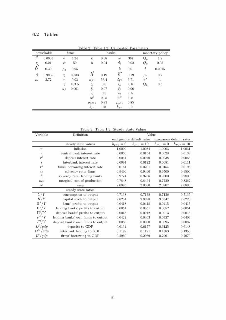
Table 2: Table 1.2: Calibrated Parametershouseholds firms banks monetary policy

rl

0.0035 θ 4.24 k 0.08 ω 367 Qp 1.2

χ 0.01 ψ 50 h 0.04 dδ 0.02 Qy 0.05

Dl

0.39 ρa 0.95 ρ 0.01 r 0.0015

β 0.9965 η 0.333 Bl

0.19 Bb

0.19 µr 0.7

m 3.72 τ 0.03 dF l 53.4 dF b 6.71 π∗ 1

γ 103.5 ζl 0.8 ζb 0.8 Qk 0.5

df 0.001 ξl 0.07 ξb 0.06

vl 0.5 vb 0.5

wl 0.05 wb 0.8

ρM(·) 0.85 ρx(·) 0.85

bF l 10 bF b 10

Table 3: Table 1.3: Steady State Values

Variable Definition Value

endogenous default rates exogenous default rates

steady state values bF (·) = 0 bF (·) = 10 bF (·) = 0 bF (·) = 10π inflation 1.0009 1.0034 1.0003 1.0031

r central bank interest rate 0.0050 0.0154 0.0028 0.0138

rl deposit interest rate 0.0044 0.0070 0.0038 0.0066

i interbank interest rate 0.0091 0.0122 0.0081 0.0111

rb firms’ borrowing interest rate 0.0161 0.0201 0.0154 0.0195

α solvency rate: firms 0.9490 0.9490 0.9500 0.9500

δ solvency rate: lending banks 0.9774 0.9766 0.9800 0.9800

mc marginal cost of production 0.7848 0.8454 0.7720 0.8362

w wage 2.0895 2.0880 2.0907 2.0893

steady state ratios

C/Y consumption to output 0.7138 0.7138 0.7136 0.7135

K/Y capital stock to output 9.8231 9.8098 9.8347 9.8220

Πf/Y firms’ profits to output 0.0418 0.0418 0.0415 0.0415

Πb/Y lending banks’ profits to output 0.0051 0.0051 0.0052 0.0051

Πl/Y deposit banks’ profits to output 0.0013 0.0012 0.0013 0.0013

F b/Y lending banks’ own funds to output 0.0422 0.0403 0.0427 0.0403

F l/Y deposit banks’ own funds to output 0.0088 0.0080 0.0095 0.0087

Dl/gdp deposits to GDP 0.6134 0.6157 0.6125 0.6148

Dbs/gdp interbank lending to GDP 0.1192 0.1121 0.1383 0.1358

Lb/gdp firms’ borrowing to GDP 0.2960 0.2969 0.2961 0.2970

21

Table 4: Table 1.4: Second Moments (Model with Endogenous Default Rates and No LeverageRatio)

Variable σπ 0.00106

K 0.21568

N 0.00264

Y 0.02222

C 0.01102

w 0.05478

gdp 0.02221

Table 5: Table 1.5: GDP and Consumption Losses for a Model with Exogenous Solvency Rates

basis scenario M bt+M

lt Mf

t xbt+xlt k (Y ) bF

bt +lF

lt

regulatory regime without leverage ratio (bF b = bF l = 0)∑


gdp-9.15% -2.70% 5.64% -8.45% -9.13% -8.52%


T−1

)12

0.471% 0.880% 0.838% 0.464% 0.470% 0.458%∑

Tt=1 βt(Ct−C)

C-2.72% -0.51% 1.00% -2.51% -2.72% -2.76%

(∑Tt=1(Ct−C)2

T−1

)12

0.240% 0.351% 0.251% 0.241% 0.240% 0.240%(∑T

t=1(πt−π)2

T−1

)12

0.231% 0.681% 0.859% 0.224% 0.236% 0.234%

regulatory regime with leverage ratio (bF b = bF l = 10)∑T

t=1 βt(gdpt−gdp)

gdp-8.74% -1.50% 5.69% -7.67% -8.70% -8.15%


T−1

)12

0.458% 0.905% 0.843% 0.449% 0.456% 0.446%∑

Tt=1 βt(Ct−C)

C-2.58% 0.11% 1.12% -2.27% -2.58% -2.63%

(∑Tt=1(Ct−C)2

T−1

)12

0.236% 0.353% 0.252% 0.236% 0.235% 0.236%(∑T

t=1(πt−π)2

T−1

)12

0.178% 0.657% 0.719% 0.175% 0.179% 0.179%

Note:

This table shows present value of GDP and consumption loss as well as variation in GDP, consumption

and inflation rate after positive shocks to default rates and subsequent central bank actions. First column

shows results for a basis scenario consisting of a positive 2,5% and 5% shocks to firm and lending banks

default rates, respectively, in a model with exogenous solvency rates. Subsequent columns present results

of quantitative easing to banks, quantitative easing to firms, qualitative easing to banks, regime switch to

output driven capital ratio and capital injection to banks, respectively, amounting to 5% of GDP each. T

= 30.

22

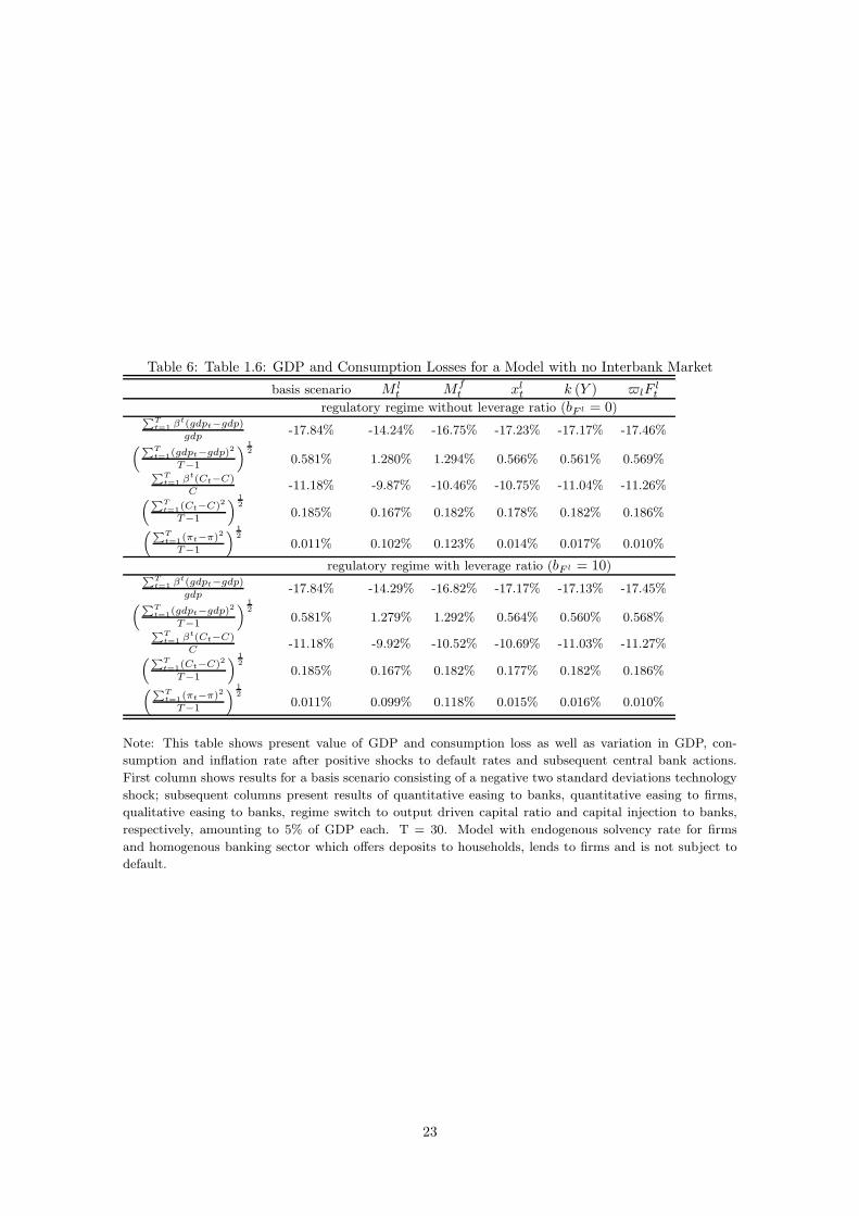
Table 6: Table 1.6: GDP and Consumption Losses for a Model with no Interbank Market

basis scenario M lt Mf

t xlt k (Y ) lFlt

regulatory regime without leverage ratio (bF l = 0)∑


gdp-17.84% -14.24% -16.75% -17.23% -17.17% -17.46%


T−1

)12

0.581% 1.280% 1.294% 0.566% 0.561% 0.569%∑

Tt=1 βt(Ct−C)

C-11.18% -9.87% -10.46% -10.75% -11.04% -11.26%

(∑Tt=1(Ct−C)2

T−1

)12

0.185% 0.167% 0.182% 0.178% 0.182% 0.186%(∑T

t=1(πt−π)2

T−1

)12

0.011% 0.102% 0.123% 0.014% 0.017% 0.010%

regulatory regime with leverage ratio (bF l = 10)∑


gdp-17.84% -14.29% -16.82% -17.17% -17.13% -17.45%


T−1

)12

0.581% 1.279% 1.292% 0.564% 0.560% 0.568%∑

Tt=1 βt(Ct−C)

C-11.18% -9.92% -10.52% -10.69% -11.03% -11.27%

(∑Tt=1(Ct−C)2

T−1

)12

0.185% 0.167% 0.182% 0.177% 0.182% 0.186%(∑T

t=1(πt−π)2

T−1

)12

0.011% 0.099% 0.118% 0.015% 0.016% 0.010%

Note: This table shows present value of GDP and consumption loss as well as variation in GDP, con-

sumption and inflation rate after positive shocks to default rates and subsequent central bank actions.

First column shows results for a basis scenario consisting of a negative two standard deviations technology

shock; subsequent columns present results of quantitative easing to banks, quantitative easing to firms,

qualitative easing to banks, regime switch to output driven capital ratio and capital injection to banks,

respectively, amounting to 5% of GDP each. T = 30. Model with endogenous solvency rate for firms

and homogenous banking sector which offers deposits to households, lends to firms and is not subject to

default.

23

6.3 Figures

Figure 5: Figure 1.5: Impulse responses after a positive technology shock

5 10 15 20 25 30−0.05

0

0.05interbank rate

5 10 15 20 25 30−0.1

0


5 10 15 20 25 30−0.1

0

0.1deposit rate

5 10 15 20 25 30−0.1

0

0.1risk−free rate

5 10 15 20 25 30−0.05

0

0.05inflation

5 10 15 20 25 300

2


5 10 15 20 25 300

2


5 10 15 20 25 30−10

0


5 10 15 20 25 30−10

0


5 10 15 20 25 300

1

2deposit supply

5 10 15 20 25 300

1

2deposit demand

5 10 15 20 25 30−1

0


5 10 15 20 25 30−1

0


5 10 15 20 25 300

0.5consumption

5 10 15 20 25 300

0.5

1capital

5 10 15 20 25 300

1

2output

5 10 15 20 25 300

0.5wage

5 10 15 20 25 30−1

0

1marginal cost

5 10 15 20 25 30−20

0

20firms profits

5 10 15 20 25 30−1

0


5 10 15 20 25 300

0.5


5 10 15 20 25 300

1

2GDP

5 10 15 20 25 30−0.2

0


5 10 15 20 25 30−0.1

0


Figure 6: Figure 1.6: Impulse responses after an expansionary monetary policy shock

5 10 15 20 25 30−0.01

−0.005

0interbank rate

5 10 15 20 25 30−0.02

−0.01

0firms borrowing rate

5 10 15 20 25 30−0.01

−0.005

0deposit rate

5 10 15 20 25 30−2

−1

0risk−free rate

5 10 15 20 25 30−0.01

−0.005

0inflation

5 10 15 20 25 30−0.2

0


5 10 15 20 25 30−0.2

0


5 10 15 20 25 30−1

0


5 10 15 20 25 30−1

0


5 10 15 20 25 30−0.2

−0.1

0deposit supply

5 10 15 20 25 30−0.2

−0.1

0deposit demand

5 10 15 20 25 300

0.5


5 10 15 20 25 300


5 10 15 20 25 300

0.005

0.01consumption

5 10 15 20 25 300

0.01

0.02capital

5 10 15 20 25 30−0.01

0

0.01output

5 10 15 20 25 300

5x 10

−3 wage

5 10 15 20 25 30−0.4

−0.2

0marginal cost

5 10 15 20 25 30−1

0

1firms profits

5 10 15 20 25 300

2


5 10 15 20 25 300

2


5 10 15 20 25 300

0.05GDP

5 10 15 20 25 300

0.005


5 10 15 20 25 30−0.01

0


24

Figure 7: Figure 1.7: Impulse responses after a liquidity injection shock to deposit banks

5 10 15 20 25 30−0.02

0

0.02interbank rate

5 10 15 20 25 30−0.05

0


5 10 15 20 25 30−0.05

0

0.05deposit rate

5 10 15 20 25 30−0.05

0

0.05risk−free rate

5 10 15 20 25 30−0.05

0

0.05inflation

5 10 15 20 25 30−10

0


5 10 15 20 25 30−10

0


5 10 15 20 25 30−20

0


5 10 15 20 25 30−20

0


5 10 15 20 25 30−2

0

2deposit supply

5 10 15 20 25 30−5

0

5deposit demand

5 10 15 20 25 30−0.1

0


5 10 15 20 25 30−0.2

0


5 10 15 20 25 30−0.05

0

0.05consumption

5 10 15 20 25 300

0.2

0.4capital

5 10 15 20 25 300

0.1

0.2output

5 10 15 20 25 300

0.05wage

5 10 15 20 25 30−0.5

0

0.5marginal cost

5 10 15 20 25 30−100

0

100firms profits

5 10 15 20 25 30−0.2

0


5 10 15 20 25 300

0.2


5 10 15 20 25 30−5

0

5GDP

5 10 15 20 25 30−0.5

0


5 10 15 20 25 30−0.5

0


Figure 8: Figure 1.8: Impulse responses after an asset swap shock to deposit banks

5 10 15 20 25 30−4

−2

0x 10

−4 interbank rate

5 10 15 20 25 30−4

−2

0x 10


5 10 15 20 25 30−4

−2

0x 10

−4 deposit rate

5 10 15 20 25 30−1

−0.5

0x 10


5 10 15 20 25 30−2

−1

0x 10

−4 inflation

5 10 15 20 25 30−0.01

0


5 10 15 20 25 30−0.01

0


5 10 15 20 25 300

0.02

0.04loans to lending banks supply

5 10 15 20 25 300

0.02

0.04loans to lending banks demand

5 10 15 20 25 30−0.1

−0.05

0deposit supply

5 10 15 20 25 30−0.1

−0.05

0deposit demand

5 10 15 20 25 300

0.005


5 10 15 20 25 300

0.1


5 10 15 20 25 300

1

2x 10

−3 consumption

5 10 15 20 25 300

1

2x 10

−3 capital

5 10 15 20 25 30−2

0

2x 10

−3 output

5 10 15 20 25 300

0.5

1x 10

−3 wage

5 10 15 20 25 30−0.01

−0.005

0marginal cost

5 10 15 20 25 30−0.1

0

0.1firms profits

5 10 15 20 25 300

0.01


5 10 15 20 25 300

0.1


5 10 15 20 25 300

2

4x 10

−3 GDP

5 10 15 20 25 30−5

0

5x 10


5 10 15 20 25 300

2

4x 10


25

Figure 9: Figure 1.9: Impulse responses after a capital injection shock to deposit banks

5 10 15 20 25 300

0.5

1x 10

−4 interbank rate

5 10 15 20 25 300

5x 10


5 10 15 20 25 300

0.5

1x 10

−4 deposit rate

5 10 15 20 25 300

1

2x 10


5 10 15 20 25 300

2

4x 10

−5 inflation

5 10 15 20 25 30−1

−0.5

0x 10

−3 loans to firms supply

5 10 15 20 25 30−1

−0.5

0x 10

−3loans to firms demand

5 10 15 20 25 30−2

−1

0x 10

−3loans to lending banks supply

5 10 15 20 25 30−2

−1

0x 10

−3loans to lending banks demand

5 10 15 20 25 300

0.01

0.02deposit supply

5 10 15 20 25 300

0.01

0.02deposit demand

5 10 15 20 25 30−4

−2

0x 10

−3 lending banks capital

5 10 15 20 25 300

2


5 10 15 20 25 30−2

−1

0x 10

−4 consumption

5 10 15 20 25 30−2

−1

0x 10

−4 capital

5 10 15 20 25 30−2

0

2x 10

−4 output

5 10 15 20 25 30−1

−0.5

0x 10

−4 wage

5 10 15 20 25 300

0.5

1x 10

−3 marginal cost

5 10 15 20 25 300

0.005

0.01firms profits

5 10 15 20 25 30−4

−2

0x 10

−3 lending banks profits

5 10 15 20 25 30−1

0


5 10 15 20 25 30−0.01

0

0.01GDP

5 10 15 20 25 30−4

−2

0x 10


5 10 15 20 25 30−4

−2

0x 10


References

Acharya, V., and H. Naqvi, 2010, The seeds of a crisis: a theory of bank liquidity and risk taking

over the business cycle, AFA 2011 Denver Meetings Paper.

Adrian, T., E. Moench, and H. S. Shin, 2010, Financial Intermediation, Asset Prices, and the

Macroecnonomic Dynamics, Federal Reserve Bank of New York, Staff Report no. 422.

Allen, F., and E. Carletti, D. Gale, 2009, Interbank market liquidity and central bank inter-

vention, Journal of Monetary Economics, 56(5), 649-652.

Angeloni, I., and E. Faia, 2010, Capital regulation and monetary policy with fragile banks,

Working paper.

Basel Committee on Banking Supervision, 2009a, The de Larosiere Group Report.

Basel Committee on Banking Supervision, 2009b, Strengthening the Resilience of the Banking

Sector.

Bernanke, B. S., M. Gertler, and S. Gilchrist, 1999, The financial accelerator in a quantitative

business cycle framework, Handbook of Macroeconomics, Amsterdam: North Holland.

Bernanke, B. S., and V. R. Reinhart, 2004, Conducting monetary policy at very low short-term

interest rates, The American Economic Review, 94(2), 85-96.

Buiter, W. H, N. Panigirtzoglou, 1999, Liquidity Traps: How to Avoid Them and How to Es-

cape Them, CEPR Discussion Papers 2203, C.E.P.R. Discussion Papers.

26

Christiano, L., R. Motto, M. Rostagno, 2010, Financial factors in economic fluctuations, ECB

Working Paper Series, No. 1192.

Christiansen, I., and A. Dib, 2008, The financial accelerator in an estimated New Keynesian

model, Review of Economic Dynamics, 11(1), 155-178.

Clarida, R., J. Gali, and M. Gertler, 1999, The science of monetary policy: a new Keynesian

perspective, Journal of Economic Perspectives, 37(4), 1661-1707.

Covas, F., S. Fujita, 2009, Time-varying requirements in a general equilibrium model of liquid-

ity dependence, Philadelphia Fed Working paper 09-23.

Curdia, V., M. Woodford, 2010, The central-bank balance sheet as an instrument of monetary

policy, Journal of Monetary Economics, forthcoming.

de Walque, G., O. Pierrard, A. Rouabah, 2009, Financial (in)stability, supervision and liquidity

injections: a dynamic general equilibrium approach, C.E.P.R. Discussion Paper No. 7202.

Derracq Paries, M., C. K. Sørensen, D. R. Palenzuela, 2010, Macroeconomic propagation un-

der different regulatory regimes: evidence from an estimated DSGE model for the euro area, ECB

Working Paper Series, No. 1251.

Dib, A., 2010, Banks, credit market frictions and business cycles, Bank of Canada, Working

Paper No. 2010-24.

Ewerhart, C., J. Tapking, 2008, Repo markets, counterparty risk and the 2007/2008 liquidity

crisis, ECB Working Paper Series, No. 909.

Faia, E., T. Monacelli, 2007, Optimal monetary policy rules, asset prices and credit frictions,

Journal of Economic Dynamics and Control, 31(10), 3228-3254.

Freixas, X., J. Jorge, 2008, The role of interbank markets in monetary policy: a model with

credit rationing, Journal of Money, Credit and Banking, 40(6), 1151-1176.

Gali, J., M. Gertler, 2007, Macroeconomic modeling for monetary policy evaluation, Journal of

Economic Perspectives, 21(4), 25-46.

Gerali, A., S. Neri, L. Sessa, F. M. Signoretti, 2010, Credit and banking in a DSGE model of

the Euro Area, Banca d’Italia, Working paper No.741.

Gertler, M., P. Karadi, 2009, A model of unconventional monetary policy, NYU, Working paper.

Gertler, M., N. Kiyotaki, 2010, Financial intermediation and credit policy in business cycle

analysis, Working paper.

27

Goodfriend, M., 2000, Overcoming the Zero Bound on Interest Rate Policy, Journal of Money,

Credit and Banking, Blackwell Publishing, vol. 32(4), 1007-35.

Goodfriend, M., B. McCallum, 2007, Banking and interest rates in monetary policy analysis:

a quantitative exploration, Journal of Monetary Economics, 54(5), 1480-1507.

Goodhart, C., P. Sunirand, D. Tsomocos, 2005, A risk assessment model for banks, Annals of

Finance, 1(2), 197-224.

Goodhart, C., P. Sunirand, D. Tsomocos, 2006, A model to analyse financial fragility, Economic

Theory, 27, 3885-3900.

He, Z., A. Krishnamurthy, 2009, A model of capital and crises, Working paper.

Hildebrand, P., 2008, Is Basel II Enough? The Benefits of a Leverage Ratio, Financial Markets

Group Lecture, London School of Economics.

Holmstrom B., J. Tirole, 1997, Financial intermediation, loanable funds, and the real sector,

The Quarterly Journal of Economics, 112(3), 663-691.

Iacoviello, M., 2005, House prices, borrowing constraints and monetary policy in the business

cycle, American Economic Review, 95(3), 739-764.

Iacoviello, M., 2010, Financial business cycles, Working paper.

Kashyap, A., R. Rajan, J. Stein, 2008, Rethinking Capital Regulation, Kansas City Symposium

on Financial Stability.

Meh, C. A., K. Moran, 2010, The role of bank capital in the propagation of shocks, Journal of

Economic Dynamics and Control, 34(3), 555-576.

Neri, S., M. Iacoviello, 2008, Housing market spillovers: evidence from an estimated DSGE

model, Banca d’Italia, Working Paper No. 659.

Smets, F., 2003, Maintaining price stability: how long is the medium term?, Journal of Mone-

tary Economics, 50, 1293-1309.

US Treasury Department, 2009, Principles for Reforming the U.S. and International Regulatory

Capital Framework for Banking Firms, Policy statement.

Walsh, C. E., 2009, Using monetary policy to stabilize economic activity, Jackson Hole Sym-

posium, 2010: 245-296.

28

munich personal repec archive - uni-muenchen.de · 0 3 5 $ munich personal repec archive...

Documents