risk aggregation in solvency ii: how to converge the ......preprint submitted on 11 jul 2009 (v1),...
TRANSCRIPT
HAL Id: hal-00403662https://hal.archives-ouvertes.fr/hal-00403662v1Preprint submitted on 11 Jul 2009 (v1), last revised 30 Jul 2009 (v2)
HAL is a multi-disciplinary open accessarchive for the deposit and dissemination of sci-entific research documents, whether they are pub-lished or not. The documents may come fromteaching and research institutions in France orabroad, or from public or private research centers.
L’archive ouverte pluridisciplinaire HAL, estdestinée au dépôt et à la diffusion de documentsscientifiques de niveau recherche, publiés ou non,émanant des établissements d’enseignement et derecherche français ou étrangers, des laboratoirespublics ou privés.
Risk aggregation in Solvency II: How to converge theapproaches of the internal models and those of the
standard formula?Laurent Devineau, Stéphane Loisel
To cite this version:Laurent Devineau, Stéphane Loisel. Risk aggregation in Solvency II: How to converge the approachesof the internal models and those of the standard formula?. 2009. �hal-00403662v1�

S
t
r
e
s
s
e
d
b
a
l
a
n
c
e
s
h
e
e
t
A
0
R
E
0
R
L
0
R
C
e
n
t
r
a
l
b
a
l
a
n
c
e
s
S
t
r
e
s
s
e
d
b
a
l
a
n
c
e
s
h
e
e
t
A
0
R
E
0
R
L
0
R
C
e
n
t
r
a
l
b
a
l
a
n
c
e
s
Risk aggregation in Solvency II: How to converge the approaches of the internal
models and those of the standard formula?
Laurent Devineau
Université de Lyon, Université Lyon 1, Laboratoire de Science Actuarielle et Financière, ISFA, 50 avenue Tony Garnier, F-69007 Lyon [email protected] Responsable R&D – Milliman Paris [email protected]
Stéphane Loisel
Université de Lyon, Université Lyon 1, Laboratoire de Science Actuarielle et Financière,
ISFA, 50 avenue Tony Garnier, F-69007 Lyon
SUMMARY
Two approaches may be considered in order to determine the Solvency II economic capital: the use of a
standard formula or the use of an internal model (global or partial). However, the results produced by
these two methods are rarely similar, since the underlying hypothesis of marginal capital aggregation is
not verified by the projection models used by companies. We demonstrate that the standard formula can
be considered as a first order approximation of the result of the internal model. We therefore propose an
alternative method of aggregation that enables to satisfactorily capture the diversity among the various
risks that are considered, and to converge the internal models and the standard formula.
KEYWORDS : Economic capital, Solvency II, nested simulations, standard formula, risk aggregation, economic ownership equity, risk factors

1. Introduction
For the purpose of the new solvency repository of the European Union for the insurance industry,
Solvency II, insurance companies are now required to determine the amount of their ownership equity,
adjusted to the risks that they incur. Two types of approach are possible for this calculation: the use of a
standard formula or the use of an internal method1.
The "standard formula" method consists in determining a capital for each elementary risk and to
aggregate these elements using correlation parameters matrices. However, the internal model enables to
measure the effects of diversity by creating a simultaneous projection of all of the risks incurred by the
company. Since these two methods lead in practice to different results (see Derien et al. (2009) for an
analysis for classical loss distributions and copulas), it seems crucial to explain the nature of the observed
deviations. This is essential, not only in terms of certification of the internal model (in relation to the
financial regulator), but also at an internal level in the Company's Risk Management strategy, as the
calculation of the standard formula must in any case be carried out, independently of the use of a partial
internal model. One must therefore be able to explain to the management or administrative body the
reason for these differences, in a manner that is understood by all, including the top ranks of the
management and the shareholders.
In this paper, we shall be analysing the validity conditions of a "standard formula" approach for both the
calculation of the marginal capital and the calculation of the global capital. We shall demonstrate that
under certain hypotheses that are often satisfied in models used by companies, the marginal capitals
according to the standard formula are very close, and sometimes identical, to those obtained with the
internal model. However, we shall also demonstrate that the standard formula generally fails in terms of
elementary capital aggregations and shows deviations in relation to the global capital calculated with the
internal model that can be significant. These differences observed in the results are mainly caused by two
phenomena:
the level of economic ownership equity is not adjusted in terms of underlying risk factors,
the "standard formula" method does not take into account the "crossed effects" of the
different risks that are being considered.
In the event of the hypotheses inherent to the "standard formula" approach not being satisfied, we
present an alternative aggregation technique that will enable to adequately comprehend the diversity
among risks. The advantage of this method is that risk aggregation with the standard formula may be
regarded as the first-order term of a multivariate McLaurin expansion series of the "economic ownership
equity" with respect to the risk factors. In some instances, risk aggregation with internal models may be
approximated by using higher order terms in addition in the expansion series. In any case, this way of
1
1 A combination of these methods may be envisaged in the case of partial internal models.

considering things enables to explain to the management body the main reasons of the difference
between the result of the standard formula and the result obtained with the internal model.
In the first part we shall discuss the issues surrounding the calculation of economic capital in the
Solvency II environment. We shall then formalise the "standard formula" and "internal model"
approaches and explain the differences on the base of projections of a savings type portfolio. In the last
but one section, we shall offer a description of our alternative aggregation method and apply it to the
portfolio being considered. Finally, we shall examine the field of application and limitations of this
approach by using another portfolio with a risk profile that makes it more complex to apply our method.

2. The calculation of the Solvency II economic capital
In this Section we offer some reminders concerning the notion of Solvency Economic Capital II and we
describe the "standard formula" approaches and the technique of "nested simulations" implemented for
the purposes of an internal model.
1. General Information
For a detailed presentation of the Solvency II economic capital calculation problematic, the reader may
consult Devineau and Loisel (2009). It is useful to remember that the Solvency II economic capital
corresponds to the amount in ownership equity available to a company facing financial bankruptcy with a
one year horizon and a confidence level of 99.5%. This definition of the capital rests on three notions:
- Financial bankruptcy : situation where the market value of the Company's assets is
inferior to the economic value of the liabilities (negative financial ownership equity),
- One year horizon: necessity of being able to carry out the distribution of the financial
ownership equity within one year,
- The 99.5% threshold: the required level of Solvency
The Solvency II capital is based on the economic balance sheet of the company as from date t=0 and as
of date t=1.
We offer here an explanation of the following notations:
- At the market value of the asset at t,
- Lt the fair value of liabilities at t,
- Et the economic ownership equity at t.
The balance sheet at takes on the following form:
Economic balance sheet at t
At Et
Lt
At the initial date of the assets' value, the liabilities and the ownership equity of the company are
determinist figures, whereas at t=1, they are random variables that depend on random (financial,
demographic...) factors that took place during the first year.
The value of each item in the balance sheet corresponds to the expected value under the risk-neutral
probability Q of discounted future cash-flows.
Denote the filtration that permits to characterise the available information for each date,

the discount factor that is expressed with the immediate risk free interest rate ru :
,
Pt the cash-flows of the liabilities (provisions, commissions, expenses) for the period t,
Rt the results of the company for period t. Equity and the fair value of the liabilities at the start date, , are calculated in the following manner:
and
In order to determine the equity and the fair value of the liabilities at t=1, a "real-world"
conditioning must be introduced for the first period. The and variables are calculated with the
expected value under the risk-neutral probability of the discounted future cash-flows, dependent of the
"real-world" information of the first year (designated as ).
This leads to the following calculations:
,
and
.
The economic capital is then evaluated with the following relation: where
P(0,1) is the price at time 0 of a zero-coupon bond with maturity 1 year.
The quantity appears as a (mathematical) surplus that needs to be added to the initial
equity in order to guarantee the following condition:
2. The standard formula
In this paper, we shall use the term "standard formula" to describe any method that aims to calculate the
economic capital at the level of each "elementary risk" (stock, rate, mortality rate,...) and then to
aggregate these capitals with correlation matrices.
A "standard formula" method may either rest on a single level of aggregation or implement successive
aggregations, as is the case for the QIS (see: CEIOPS QIS 4 Technical Specifications 2008). In fact, this
method consists in aggregating, in a first stage, the elementary capitals within different risk modules
("market" module, "life" module, "non-life" module,...) This phase corresponds to an intra-modular
aggregation. The capitals of each module are then aggregated, so as to obtain the global economic

capital (inter-modular aggregation). It should be noted that both the GCAE (2005) and Filipovic (2008)
underline the limits of such an approach2.
A "standard formula" type method corresponds to a bottom-up approach to risks (i.e. starting with the
elementary risks and ending with the calculation of the global capital). The calculation of the elementary
capitals implies the use of an ALM model that provides a financial balance sheet as from the start date.
This model enables, amongst other things, to calculate the amount of "central" economic equity, i.e. the
equity according to the terms in effect on the calculation date, as well as the economic equity resulting
from an instantaneous shock of these conditions.
More precisely, to calculate the elementary capital for the purpose of risk R, an instantaneous shock
is delivered to the R factor, and the economic equity is determined after the shock. This amount is
then subtracted from the central economic equity in order to obtain the economic capital for the
purpose of R.
In order to determine , the calculations must be reconditioned with a new filtration in mind,
which derives from the instantaneous shock on the R factor. The ALM model is used to estimate the
following quantity:
where corresponds to the risk-neutral probability that is applied to filtration .
The elementary capital is then represented as
.
The following diagram illustrates the calculation method of the elementary capital in terms of Risk R.
Figure: calculation of the elementary capital in terms of risk R with the "standard formula" method.
2 Filipovic demonstrates that the correlation factors that enable to carry out the inter-modular aggregation
are in fact dependent on the company's specificities. Therefore, since it is impossible to use a "benchmark" correlation matrix, this approach loses its universal characteristic.
Stressed balance sheet
Central balance sheet

Note that (resp. ) represents the market value of the assets (resp. the fair value of the liabilities) at
0 after the shock on the R factor.
In order to estimate quantities and , Monte-Carlo simulations are carried out. The following
notation should be introduced at this point, in order to formalise the calculations performed according to
the ALM method.
Write (resp. ) the result of date for the simulation according to Q (resp.
under ), and
(resp. ) the discount factor of the date for the s simulation under Q (resp. under ).
The amounts of and are then estimated in the following manner:
and
Comment: for the purpose of coherence with the definition of the Solvency II economic capital, the
instantaneous shocks delivered to the various elementary risks are homogeneous in terms of extreme
deviations (i.e. the 0.5% or 99.5% threshold depending on the "sense" of risk) according to the physical
probability.
The elementary capitals are then aggregated with correlation matrices. Let us define
all risks of module m,
the capital for the purpose of risk i,
the correlation coefficient that enables to aggregate the capitals of risks i and j belonging to
module m,
the economic capital (designated as Solvency Capital Requirement) of module m,
M the number of modules,
the correlation coefficient that enables to aggregate the capitals of modules i and j,
the global economic capital (designated as Basic Solvency Capital Requirement) before
operational risks and adjustments.
A QIS type aggregation is based on two main stages:
- An intra-modular aggregation: for each risk module m, the economic capital SCRm is
calculated in the following manner :
- An inter-modular aggregation: the BSCR global capital is obtained by aggregating the
capitals of the different modules.

Intra-modular aggregation
Inter-modular aggregation
Bo
tto
m-u
p a
gg
reg
atio
n
- Hereunder is the mapping that was chosen for the calculation of the economic capital QIS 4:
-
Figure: mapping of the risks of the QIS 4
Comment: in a "standard formula" approach, the calculations are often carried out at the initial date.
Therefore, the economic capital does not rest on the distribution of equity at the end of the first year but
rather on the elementary capitals determined at t=0.
On the other hand, an internal model that performs NS projections (Nested Simulation) enables to
calculate the economic capital by complying with all the Solvency II criteria.
3. The Nested Simulations (NS) method
As we have seen above, the Solvency II economic capital is described in relation to the 0.5% quantile of
the distribution of equity at the end of the first year and of the amount of economic equity at the start
date. The link between these various elements is provided by the following relationship:
There are generally no operational issues in the determination of the quantity; all that is needed to
obtain this quantity is an ALM model that enables to carry out "market consistent" valorisations at t=0.
However, it is more delicate to obtain the distribution of the variable, and the calculation of the
economic equity at t=1 is required, conditional on the hazards of the "real-world". The "Nested
simulations" technique (NS) enables to address this problematic. To this date, this application is one of
the most compliant methods with the Solvency II criteria for annuity products. Devineau and Loisel
(2009) offer a detailed description.

Balance sheet at t=1 – simulation i
Balance sheet at t=1 – simulation P
Simulation i
Simulation P
Simulation 1
E11
L11
t = 0 t =1
Secondary simulations “market consistent”Primary simulations “real world”
A1i E1
i
L1i
Balance sheet at t=1 – simulation 1
A11
A1P E1
P
L1P
…
…
Balance sheet at t=0
A0 E0
L0
Balance sheet at t=1 – simulation i
Balance sheet at t=1 – simulation P
This method consists in carrying out, through an internal model, "real-world" simulations on the first
period (called primary simulations) and launching, at the end of each one of these simulations, a set of
new simulations (called secondary simulations), in order to determine the distribution of the economic
equity of the company at t=0. The secondary simulations have to be "market consistent"; in most cases
these are risk-neutral simulations.
In order to formalise the calculations carried out in a NS approach, let us define
the result of the u>1 date for the primary simulation, , and for the secondary
simulation,
the result of the first period for the primary simulation p,
the discount factor of the u>1 date for the primary simulation, p, and for the secondary
simulation, s,
the discount factor of the first period for the primary simulation, p,
the information of the first year contained in the primary simulation, p,
the economic equity at the end of the first period for the primary simulation, p,
the fair value of liabilities at the end of the first period for the primary simulation, p,
the market value of the assets at the end of the first period for the primary simulation, p.
This application may be seen in the following diagram:
-
Figure : obtaining the distribution of economic equity with the NS method.
The economic equity at t=1, for the primary simulation, p, satisfies

For the calculation of , the following estimator is considered:
The determination of the , quantity is generally based on the estimator. In other
words, the "worst value" of the sample is taken as estimator of
The economic capital is then evaluated with the estimator: .
3. Formalising the "standard formula" and "NS" approaches
In this section, we propose a formalisation of the "standard formula" and NS approaches. First we shall
introduce the notion of risk factors, which we associate with "standard formula" shocks and with the
primary simulations of a NS projection. Then we shall adapt the definition of the economic capital
calculation so as to return to an analysis over a single period, which enables to compare the results of the
"standard formula" and those of the internal model. Finally, we shall establish the theoretical framework
that legitimises the marginal and global capitals obtained with the "standard formula" method. The
partial internal models presented herein are of the same type as those used by companies. We are aware
of the limits of these models. It would be a good idea to perfect them, but that is not the object of this
paper: our aim is to study the risk aggregation issues in partial internal models typically used by
insurance companies.
1. Risk factors
Risk factors are elements that enable to summarise the intensity of the risk for each primary simulation
in an NS projection. For example, let us suppose that the stock is modelled according to a geometric
Brownian motion; in this case, the risk factor that one can consider is that of an increase of the Brownian
motion of the diffusion over the period in question. Very low values for these increases correspond to
cases where the stock is submitted to very strong downward shocks (adverse situation in terms of
solvency).
It is possible to extract the risk factors from a table of economic scenarios for the first period by
specifying an underlying model for each risk and by evaluating the parameters of each model. We shall
describe this approach as an "a posteriori determination method" 3.
3 When the company has a precise knowledge of the underlying risks' modelling and simulates its own
trajectories, it is sufficient to export all the simulated random events when the primary trajectories are generated. Amongst other things, this enables to realise the increase of Brownian motions of the diffusions (rate, stock,...). In this case, the factors are known before the modelling.

In the example that we offer as part of the fourth section "Application: comparison of the standard
formula and NS approaches", we follow an a posteriori approach based on the first year "real-world"
table used for NS projections.
From now on in this Section, write
the stock at t,
a random variable distributed according a Normal-Inverse Gaussian distribution
,
a centred and standard normal distribution,
the price at t of a zero-coupon bond for a currency as of date T>t, The real-world return of the zero-coupon bond with a maturity T,
The real-world volatility of the zero-coupon bond with a maturity T,
ρ the Pearson's correlation coefficient of variables and .
We shall suppose that the evolution of the value of stock and the price of zero-coupon bonds in a "real-
world" environment for the first year is described by
(1)
and
(2)
Relation (1) corresponds to a modelling of the stock price according to an exponential NIG-Levy process.
For a detailed description of this type of model, see Papapantoleon (2008).
Relation (2) is derived from a linear volatility HJM (Heath-Jarrow-Morton) type model4.
Evaluation of the parameters
Let be the stock price at date 1 in primary simulation p and
be the price at t of a zero-coupon bond for a currency as of date T in simulation p. The interest rate parameters are evaluated from the economic scenarios' table of the first period.
In order to evaluate the parameters of the stock price model, we present hereunder a reminder of the
properties of a distribution. With we obtain:
-
4 See Devineau et Loisel (2009)

-
-
- and
where (resp. ) represents the skewness coefficient (resp. Kurtosis excess coefficient) of the
distribution.
Let (resp. ) be the empirical estimator of the expected value (resp. the variance, the
skewness, the kurtosis excess) calculated for the sample.
The density of is expressed as follows:
where K1 is a Bessel function of the third kind with parameter 1.
First, an estimation of the moments of parameters α,β,δ,μ is to be carried out by minimisation of the
criteria
.
We shall then determine the estimator of maximum likelihood for α,β,δ,μ by initialising the optimization
algorithm with the moments' estimator obtained above.
Extraction of stock and zero-coupon bond related risk factors
For each primary simulation p, we shall establish the pair of centred and reduced random
events, using the estimators presented above:
and

2. The global and marginal NS projections
The NS method described above enables us to determine the global economic capital of the company.
However, in order to compare the NS and "standard formula" approaches, it might be useful to know, in
addition to the global capitals, the value of the elementary capitals. This will enable to determine if the
differences noted between the two methods are due to elementary capitals or to the aggregation
method (or both).
Definitions:
- We shall use the term marginal scenarios for risk R to describe a set of primary
simulations, for which all the random events are cancelled out, except for the random event
pertaining to R.
- We shall use the term Marginal NS in terms of risk R to describe any NS projection for
which the primary scenarios are the marginal scenarios of risk R.
It is thus possible to determine the 0.5% level quantile of the economic equity distribution at t=1
conditional on risk R, by performing a marginal NS. Where is the estimator of the said
quantile.
It is then easy to obtain the marginal economic capital CR in terms of risk R from the following relation:
3. "Standard formula" vs internal model
The results of the standard formula and the internal model can be analysed on two levels:
- Marginal level: comparison of the "standard formula" capital determined by stress test
and the capital calculated according a marginal NS,
- Global level: in the case where the marginal capitals obtained with the "standard
formula" are very close or identical to those obtained with the internal model, comparison of the
"standard formula" aggregation method and the NS method.
Hereunder is a recall of the diagram showing the marginal capital calculation in terms of R using the
standard formula:

AR,p(1) ER,p(1)
LR,p(1)t=0 t=1
E0
L0
A0
Simulation p
Balance sheet at t=0 Balance sheet at t=1
Figure: calculation of the elementary capital in terms of risk R with the "standard formula" method.
Hereunder we also present a figure showing the calculation of the capital in terms of risk R using a
marginal NS:
Figure : calculation of the NS marginal capital relating to risk R.
Where the primary simulation p is the simulation associated with the 0.5% level quantile of the
variable that represents the distribution of economic equity at t=1, conditional only on risk R.
Two fundamental differences are observed in terms of marginal capitals between the "standard formula"
and internal model approaches:
- Calculation timing: the "standard formula" approach consists in comparing the value of
the economic equity before and after the shock at t=0, whereas the calculation using the
marginal NS is based on the discounted quantile of the equity at then end of the first period.
- The "standard formula" method uses a valorisation after shock (notion of quantile on the
R risk factor), whereas the "Marginal NS" method rests on marginal simulations of economic
equity (notion of quantile on the distribution of economic equity).
In order to compare the results of the "internal model" and those obtained with the single period
"standard formula" approach, we shall slightly amend the latter by modifying our definition of economic
capital.
- We shall then place ourselves in a single period context and we shall describe the
following value as economic capital:
Stressed balance sheet
Central balance sheet

A1R E1
R
L1R
t=0 t=1
E0
L0
A0 « standard formula »
shock
Balance sheet at t=0 Balance sheet at t=1
where represents the value of economic equity at t=1, when all the random events of the
first period have been cancelled out. This relation enables to define the global capital and the
marginal capital, the calculation of which can be carried out using a "NS (global or marginal)"
method.
- Rather than performing an instantaneous stress test for the determination of the
marginal capital in terms of risk R with the standard formula, we shall apply the corresponding
shock to the first period by cancelling out all the other sources of random events. The marginal
capital will thus be the difference between the centre value and the level of economic
equity at t=1, conditional on the "standard formula" shock (noted ):
The following diagram illustrates the change of shock timing in the "standard formula" method:
-
Illustration : adapting of the shock timing in the "standard formula" method.
On the basis of these adjustments, we shall propose in the following section a theoretical analysis of the
"standard formula" approach.
4. Theoretical analysis of the "standard formula" approach
In this section we describe the theoretical framework required to calculate the economic capital with the
"standard formula" method.
4.1. Case of an elementary capital
In this Section, we shall assume that risk R may be entirely characterised by a risk factor that we shall
denote as .
Note that in a marginal NS projection in terms of R, the value of economic equity at t=1 is a function of
the risk factor .
In other words, if designates the value of the risk factor in the primary situation p, then:
By taking α=0.5% or α=99.5% as functions of the "sense" of risk R, then the calculation of the CRSF
economic capital can be described as

whereas an approach of the marginal NS type would give the following capital:
.
In the above expression, the quantile is considered on the "economic equity" function of the factor
and not on the factor itself.
The analysis of the "standard formula" vs the internal model therefore consists in comparing elements
and
In order to compare these elements, let us introduce the following H0 hypothesis:
H0 : the amount of economic equity at t=1 is a monotonic function of the risk factor εR.
According to H0, there are two scenarios. These are as follows:
f is a decreasing function5 :
f is an increasing function:
H0 is a very strong hypothesis. In some cases, economic equity may be penalised for both very low and
very high values of the risk factor .
As an example of this, consider an annuity product with a significant guaranteed interest rate and with a
dynamic lapses' rule. The economic equity will be degraded for both low and high values of the "interest
rate" risk factor and its monotonic nature will not be verified. It is possible to relax the H0 hypothesis by
considering the H0bis hypothesis, which we shall designate as hypothesis of predominance.
H0bis : hypothesis of predominance
If one assumes that the "economic equity" function:
– is decreasing (resp. increasing) beyond the q-quantile, where q<98%, say, (resp. before q-quantile with q<2%, say) of the risk factor, – and takes on higher values when the factor is below (resp. above) the q-quantile,
1 With
Where

R
f( R)
q99,5%( R)
Figure : profile of the "economic equity" function according to the hypothesis of predominance.
then:
The hypothesis of predominance consists in considering that the situations of bad solvency are explained
by extreme values taken on by the risk factor "in any direction" (upwards or downwards). Statistical
issues about tests of Hypothesis H0bis are left for future research.
The monotonic hypothesis, also called the hypothesis of the predominance of the "economic equity" function in terms of the risk factor, justifies the fact that the quantile approach on equity is equivalent to the quantile approach on risk factor.
4.2. Analysis of the risk aggregation method
The technique of risk aggregation using a correlation matrix rests on a Markowitz mean-variance type
approach. This method of aggregation is described, amongst other authors, by Saita (2004) and by
Rosenberg and Schuermann (2004). The latter describe in their paper the case of the VaR of a portfolio
containing three assets; the approach can be broadened to the calculation of the VaR of economic equity,
depending on the different risk factors.
Aggregation techniques are often based on the notion of an economic capital that corresponds to the
difference between the quantile and the expected value of a reference distribution (value of the
portfolio, amount of losses, equity level,...). In our case, and using, for the purpose of simplifying the
notations, E to describe the end of period economic equity, this definition leads to the following amount
C of economic capital:
,
where is the expected value of variable E.
-
We shall use this hypothesis to demonstrate the "standard formula" aggregation method under certain
hypotheses.

A pre-requirement for the application of this method is that the global variable (annuity of the asset
portfolio, economic equity of the company) is a linear function in terms of drivers (annuities of the
portfolio's assets, risk factors,...). This is indeed the hypothesis that will enable to calculate de variance of
the interest rate variable in relation to the variance and covariance of the drivers.
We shall then assume that the company is exposed to three risks, X, Y, Z and that the distribution of
economic equity at t=1 is linear for each one of these factors:
with and
Hereunder we shall use notation (resp. ) to describe the expected value (resp. the standard
deviation) of a random variable M.
The coefficient will describe the linear correlation (Pearson's coefficient) between the two variables
M and N.
We shall assume in this Section that variables E, X, Y and Z have finite moments of the second kind. First,
let us calculate the variance of E :
Let M be a random variable with expected value and standard deviation . We shall use M to
describe the reduced and centred variable
We obtain the following relation:
Consequentially, by using the expression of the variance of E in relation to the variance and correlation
coefficient of each one of the 3 drivers X, Y and Z, one obtains:
In the case of an extreme quantile (α=0.5%), the value of the normalised distribution's quantile is
therefore negative:

In Appendix 2 we recall that when the random vector is elliptic6, one obtains the following
result:
which leads to the C capital hereunder:
Where (resp. , ) corresponds to the economic capital in terms of risk X (resp. Y, Z), and
is the sign of .
In the event of all the coefficients all having the same sign, the QIS aggregation relation is found.
Comment: it is always possible to return to risk factor coefficients that have the same sign, even if this
entails considering the opposites of the risk factors. However, in this instance, the correlations change
sign.
It should be reminded that the establishment of this relation required the hypotheses hereunder.
H1 : the E variable is a linear function of variables X, Y and Z,
H2 : the vector follows an elliptic distribution (e.g. normal or Student distribution).
Comments:
- The H1 hypothesis ensures the standard nature of the correlation coefficient. Indeed, if the "economic equity" function is not linear in terms of risk factors, the linear correlations of the marginal distributions of economic equity are, generally speaking, different from those of the factors7. These parameters are no longer "market" values since they become "company" values (and therefore the "standard formula" approach loses its universal nature).
6
1 Gaussian and multivariate Student distributions are well known examples of elliptic distributions. For a
detailed description of these distributions, see Appendix 1. 7
7 The linear correlation is not invariant by increasing transformations, contrary to a Kendall tau rank
correlation coefficient.

- The H2 hypothesis imposes a constraint on both the marginal distributions and the copula that links them. In other words, all marginal distributions must be identical and belong to the same family as the copula. In practice, this means considering the two most standard cases:
o marginal distributions and Gaussian copulas o marginal distributions and Student copulas
4. Application: comparing the "standard formula" and "NS" approaches
In this Section we shall present, for a savings type portfolio, a comparison of economic capitals obtained,
on one hand with the "standard formula", and on the other with the internal model. To begin with, we
shall restore the results obtained from global and marginal NS projections, and we shall compare these to
the aggregated and elementary capitals obtained with the "standard formula". We shall then propose a
deviations' analysis that will enable to explain in large part the noted differences.
1. Description of the portfolio and of the model
The portfolio that we consider in this study is a savings' portfolio with no guaranteed interest rate. We
have projected this portfolio using an internal model that performs ALM stochastic projections and the
calculation of economic equity after one year. This projection tool enables the modelling of the profit
sharing mechanism, as well as the modelling of behaviours in terms of dynamic lapses of the insured
parties when the interest rates handed out by the company are deemed insufficient in relation to the
reference interest rate offered by the competitors.
In this study, are considered only the stock and interest rate related risks. The tables of economic
scenarios that are used were updated on December 31, 2008. Let's note that the implicit "stock" and
"interest rate" volatility parameters have been assumed as being identical for each set of "risk-neutral"
secondary simulations. However, one should note that it is possible, in a NS application, to jointly project
the risk factors and implicit volatilities on the first period, and to reprocess the market consistent
secondary tables in relation, inter alia, to simulated volatilities. This approach would make it possible to
take the implicit volatility risk into account, as suggested by the CRO Forum (2009).
The company's economic balance sheet at t=0 is as follows:
Asset market value - A0 360 754
Fair value of the liabilities - L0 353 394
Economic equity - E0 7 360 Table: economic balance sheet of the company at t=0 (in M€)
The investment strategy at time 0 is as follows :

-5
-4
-3
-2
-1
0
1
2
3
4
5
-6 -4 -2 0 2 4
Cash 5%
Stock 15%
Bonds 80% Table: distribution of the assets at market value at t=0
2. Results
2.1. Risk factors
The extraction of risk factors according to the method described above leads to the following cloud:
-
Figure : risk factor pairs relating to stock (abscissa) and zero-coupon bonds (ordinate)
Each point in the cloud corresponds to a primary simulation. In the graph hereunder, we present
descriptive statistics pertaining to stock and zero-coupon bonds (noted ZC) related risk factors.
Stock risk factor ZC risk factor
Expected value
0.0 0.0
Std error 1.0 1.0
Skewness -0.5 0.0
Kurtosis 0.7 -0.1 Table : statistical indicators of samples et
Pearson's correlation coefficient for stock factors and zero-coupon bonds' factors is the following:
.
These two distributions are centred and reduced but the stock distribution shows kurtosis and skewness
coefficients that are significantly different from those found in a normal distribution. This is due to the
fact that the log-increase of the stock follows an inverse Gaussian Normal distribution The graph
hereunder shows that the variable takes on more extreme negative values than the variable.
Indeed, the distribution is asymmetrical with a heavy tail, whereas the follows a centred and
reduced normal distribution.
0%
1%
2%
3%
4%
5%
6%
7%
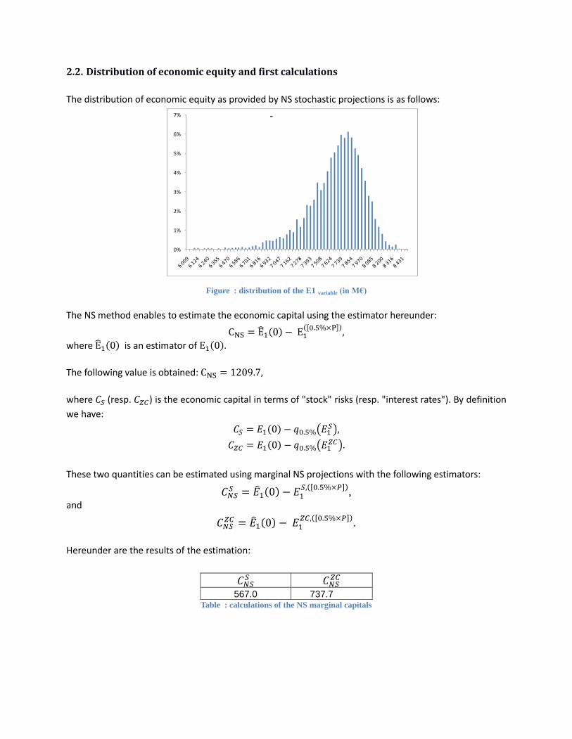
2.2. Distribution of economic equity and first calculations
The distribution of economic equity as provided by NS stochastic projections is as follows:
-
Figure : distribution of the E1 variable (in M€)
The NS method enables to estimate the economic capital using the estimator hereunder:
where is an estimator of
The following value is obtained:
where (resp. ) is the economic capital in terms of "stock" risks (resp. "interest rates"). By definition
we have:
These two quantities can be estimated using marginal NS projections with the following estimators:
,
and
.
Hereunder are the results of the estimation:
567.0 737.7 Table : calculations of the NS marginal capitals

6300
6500
6700
6900
7100
7300
7500
7700
7900
8100
8300
-6 -5 -4 -3 -2 -1 0 1 2 3 4
3. Analysis of the deviations
3.1. Comparison of stand-alone capitals
As has been demonstrated above, the comparison of "standard formula" and internal model approaches
means to compare respectively the elements and , where f is the "economic
equity" function and α=0.5% or α=99.5% is a function of the "sign" of risk R.
Since the "stock" related risk is a decreasing risk, elements and are
compared hereunder.
For the purpose of our research, the following equality is used:
Therefore, the "standard formula" approach (equity governed by the risk factor quantile) and the internal
model approach (quantile on the distribution of economic equity) coincide.
Hereunder, we present the profile of in relation to the value of the risk factor :
- -
-
-
-
-
-
-
-
-
-
-
-
-
-
-
-
-
-
Figure: Value of in relation to the level of risk factor
As this is an increasing function, Hypothesis H0 is verified and the "standard formula" and internal model
approaches are equivalent.
The graph hereunder presents the marginal economic equity in terms of the value of the risk factor
:

6300
6800
7300
7800
8300
-5 -4 -3 -2 -1 0 1 2 3 4 5
Figure : Value of in relation to the level of risk factor
One notes that it is the very low values for that lead to the most adverse situations in terms of
solvency. One should remember that a low value corresponds to the case where the price of zero-
coupons falls and therefore the interest rates increase. This corresponds to the product under
consideration as it is exposed to an increase of the interest rate (triggering of a wave of dynamic lapses).
For the purpose of this study, we must therefore compare the elements
and .
We find and .
There is a 0.4% difference between these two amounts.
Although these two values are very close, they are not identical since the extraction of zero-coupon
bonds related risk factors induces a specification error. The deformation of the price of zero-coupon
bonds is summarised independently from the maturities by a single random event, whereas the
underlying model is generally far more complex.
However, one may observe that the value of marginal equity rises globally along with the risk
factor.
The linear nature of the variable in terms of the "stock" risk factor is acceptable with regard to graph
10. However, graph 11 contradicts the linear nature of in terms of risk factor . The H1 hypothesis
(assuming a linear relation between economic equity and risk factors) is therefore not verified and the
aggregation of the "standard formula" is compromised in such a context.
3.2. Comparison of global capitals
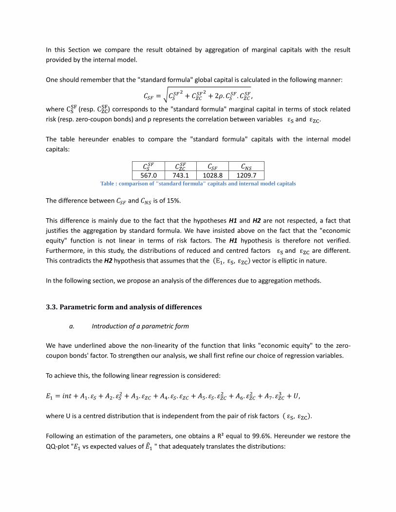
In this Section we compare the result obtained by aggregation of marginal capitals with the result
provided by the internal model.
One should remember that the "standard formula" global capital is calculated in the following manner:
,
where (resp. ) corresponds to the "standard formula" marginal capital in terms of stock related
risk (resp. zero-coupon bonds) and ρ represents the correlation between variables and .
The table hereunder enables to compare the "standard formula" capitals with the internal model
capitals:
567.0 743.1 1028.8 1209.7 Table : comparison of "standard formula" capitals and internal model capitals
The difference between and is of 15%.
This difference is mainly due to the fact that the hypotheses H1 and H2 are not respected, a fact that
justifies the aggregation by standard formula. We have insisted above on the fact that the "economic
equity" function is not linear in terms of risk factors. The H1 hypothesis is therefore not verified.
Furthermore, in this study, the distributions of reduced and centred factors and are different.
This contradicts the H2 hypothesis that assumes that the vector is elliptic in nature.
In the following section, we propose an analysis of the differences due to aggregation methods.
3.3. Parametric form and analysis of differences
a. Introduction of a parametric form
We have underlined above the non-linearity of the function that links "economic equity" to the zero-
coupon bonds' factor. To strengthen our analysis, we shall first refine our choice of regression variables.
To achieve this, the following linear regression is considered:
,
where U is a centred distribution that is independent from the pair of risk factors .
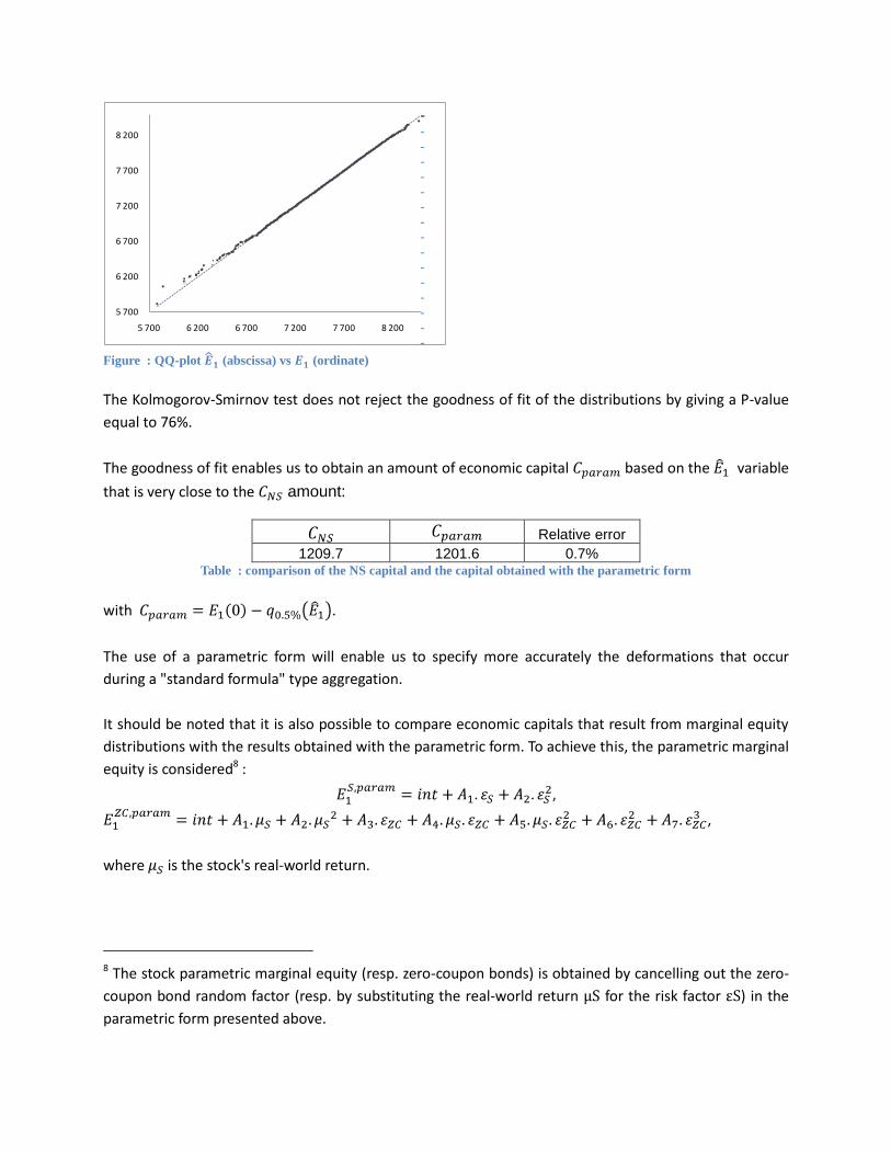
Following an estimation of the parameters, one obtains a R² equal to 99.6%. Hereunder we restore the
QQ-plot " vs expected values of " that adequately translates the distributions:
5 700
6 200
6 700
7 200
7 700
8 200
5 700 6 200 6 700 7 200 7 700 8 200
- -
-
-
-
-
-
-
-
-
-
-
-
-
-
-
Figure : QQ-plot (abscissa) vs (ordinate)
The Kolmogorov-Smirnov test does not reject the goodness of fit of the distributions by giving a P-value
equal to 76%.
The goodness of fit enables us to obtain an amount of economic capital based on the variable
that is very close to the amount:
Relative error
1209.7 1201.6 0.7% Table : comparison of the NS capital and the capital obtained with the parametric form
with .
The use of a parametric form will enable us to specify more accurately the deformations that occur
during a "standard formula" type aggregation.
It should be noted that it is also possible to compare economic capitals that result from marginal equity
distributions with the results obtained with the parametric form. To achieve this, the parametric marginal
equity is considered8 :
,
where is the stock's real-world return.
8 The stock parametric marginal equity (resp. zero-coupon bonds) is obtained by cancelling out the zero-
coupon bond random factor (resp. by substituting the real-world return μS for the risk factor εS) in the
parametric form presented above.

6 600
6 800
7 000
7 200
7 400
7 600
7 800
8 000
8 200
6 600 6 800 7 000 7 200 7 400 7 600 7 800 8 000 8 200
6 400
6 600
6 800
7 000
7 200
7 400
7 600
7 800
8 000
8 200
6 400 6 600 6 800 7 000 7 200 7 400 7 600 7 800 8 000 8 200
The QQ-plots hereunder for (resp. ) vs (resp. ) show a very good fit for the
distributions:
- -
-
-
-
-
-
-
-
-
-
-
-
-
-
-
-
Figure : QQ-plot (abscissa) vs (ordinate)
-
Figure : QQ-plot (abscissa) vs (ordinate)
The goodness of fit is also measured by the P-value of the KS-test, equal to 39% (resp. 19%) for "Stock
equity (resp. zero-coupon bonds)".
Let (resp. ) be the "stock" marginal capital (resp. zero-coupon bonds) calculated with the
variable (resp. ). One obtains:
and

The parametric approach provides an estimation of the marginal capitals that is very close to the results
obtained with marginal NS projections:
Difference
567,0 555,9 2,0% Table : comparison of "NS" and "parametric" stock marginal capitals
Difference
737,7 723,6 1,9% Table : comparison of "NS" and "parametric" zero-coupon bonds' marginal capitals
Since the results of the NS projections are very close to those obtained with the parametric form, we
shall use the latter as basis in the rest of this section. The parametric structure will indeed enable us to
explain the deviations noted between "standard formula" economic capitals and "internal model"
economic capitals, based on crossed factors of the or type.
b. Analysis of the deviations
Consider the following variable:
The variable specifically integrates the crossed terms ou .
We shall designate the economic capital in terms of crossed effects as . It is defined by the
following relation:
We obtain a linear relation between the variable and the marginal distributions of vector
:
If the distribution of vector belongs to the same family of elliptic
distributions, the global capital (noted ) may be calculated as follows:
where
is the linear correlation between variables and ,
is the linear correlation between variables and ,
And is the linear correlation between variables and .

Comment: a "standard formula" type method fails to capture the "crossed" effects or , since
isolating the risks implies cancelling out one of the two factors ( ou )
A "standard formula" method therefore consists in performing the following calculation:
This approach therefore underestimates the risk when:
Hereunder are the obtained results:
Stand-alone capitals:
555.9 723.6 227.6
Table : marginal capitals associated to variables and
Correlation matrix:
1 21.5% 40.2%
21.5% 1 32.5%
40.2% 32.5% 1
Table: correlation matrix of vector
Capital aggregated using the previous correlations
Capital CSF « standard formula » on
1002.9
Capital C2 sur
1225.4
1201.6
Table : capitals associated with risks and
The difference between the capital and the capital obtained by aggregation of risks
is significant (16.5%). This is due to the fact that the risk inherent to crossed variables
is not integrated in the calculation. By taking this risk into account in the C2 calculation based on
, the difference is reduced from 16.5% to 6.3% in relation to the
reference capital .

-15,0
-13,0
-11,0
-9,0
-7,0
-5,0
-3,0
-1,0
1,0
3,0
5,0
-9 -7 -5 -3 -1 1 3
Calculationbased on the
equity distribution
Standard Formula aggregation
Stock x ZC x Cross-terms
Standard Formula aggregation
Stock x ZC
Stock risk
ZC risk
Cross-terms risk
Non elliptical distributions
Cross-terms not taken into account in the QIS
However, as the linear hypothesis is verified ( is a linear function of variables , and
), the residual error is explained by the non-elliptic nature of the distribution.
Consider the QQ-plot of standard distributions (i.e. centred and reduced) of and :
- -
-
-
-
-
-
-
-
-
-
-
-
-
-
-
Figure : QQ-plot of standard distributions of and
The above graph reveals that the reduced and centred marginal distributions of vector
do not follow identical distributions. The latter's elliptic nature is
therefore contradicted.
The following diagram offers a summary of the deviations between capitals obtained with the standard
formula and those calculated with the internal model:
-
Figure : summary of the differences between "standard formula" capitals and internal model capitals
-

5. Alternative aggregation method
The principle behind this method is to infer the results obtained with the parametric model9 in the risk
aggregation method. We have observed above that the calculation of the global capital by aggregation in
a non-linear situation lead to a different amount than that found with the "internal model" . This is
essentially due to the or crossed variables that are not taken into account (as they are
cancelled out in succession) in the "standard formula" approach. The sole use of marginal capitals is
therefore not sufficient to satisfactorily measure the effects of diversification.
In order to capture this phenomenon, without necessarily using an entirely integrated NS internal model
(relatively complex modelling), we propose a method that is easily implemented and based on an ALM
projection tool that enables to carry out valorisations only at t=0.
1. Description of the method
We shall detail here the principle stages of the alternative method:
Stage 0 - determination of the marginal capitals:
Calculation of the stand-alone capitals of each risk factor (by variation of the economic equity at t=0 due
to an immediate shock on a risk factor).
Stage 1 - obtaining an equity distribution:
Step 1 : establishment of risk factors' tuples (stock, interest rate, mortality,...) These
tuples are not necessarily vectors created from simulations and they can be established
"manually". Each tuple represents a deformation of the initial conditions.
Step 2: calculation of the amounts of the equity in relation to each tuple, using the
projection model at t=0.
Step 3: calibration of a parametric form of the "equity" variable on the previous tuples.
Step 4: simulation of the risk factors (modelling of marginal distributions and of the
copula that links them together).
Step 5: obtaining the equity "distribution" using the previous simulations and the
parametric form calibrated in Step 3.
Stage 2 - adjustment of the correlations that reveal the "non-linear" diversification:
Consider three risks, X, Y and Z to describe this point.
9
9 on the basis of a calibration that requires few observations (see hereunder)

The capital calculated on the basis of the distribution in phase 5 is noted and the elementary
capitals calculated from the parametric form (by cancelling out all the other risks) are noted
, , . If R is the correlation matrix that enables to reproduce the non-linear
diversification, one obtains:
. (*)
The minimal standard R, for which (*) is respected, is found. This leads to the following optimisation
program:
under the constraint (*),
with
Stage 3 - calculation of the global capital that integrates the "non-linear" diversification:
If are the elementary capitals calculated in stage 0, the global capital is determined
with the following relation:
Comments:
- When only risks X and Y are considered, the constraint (*) has a single solution:
- The coefficients of the matrix enable to "reproduce" the effects of the diversification
that are due to the parametric form but they do not correspond, generally speaking, to the
correlation coefficients. These adjustment factors are used in order to integrate the marginal
capitals by using the standard formula, but in no case are these Pearson's correlation coefficients
of underlying variables10.
10
10
In some cases, they can be greater than 1 in absolute value.

-5
-4
-3
-2
-1
0
1
2
3
4
5
-6 -5 -4 -3 -2 -1 0 1 2 3 4
2. Implementing the alternative method
In the section concerning the analysis of deviations, the calibration of the function linking economic
equity and risk factors is based on all of the 5000 primary simulations. A comprehensive NS projection
was therefore carried out to calibrate this function.
However, it is often operationally difficult to carry out such a large number of simulations as these imply
significant computation times. Devineau and Loisel (2009) have developed an acceleration algorithm that
enables to reduce the number of primary simulations in a NS calculation.
The principle consists in calculating for each primary simulation the standard11 that is associated with the
underlying risk factors and then performing NS projections in a decreasing order until reaching the
stability of the worst values of economic equity.
The NS accelerator converges after 300 primary simulations on the portfolio under consideration. In this
section, we have taken the parametric structure introduced above and calibrated it on the basis of the
300 pairs of factors on the biggest standards. This enables to adjust the parametric form on the extreme
quantiles of the economic equity distribution, as the calculation of the economic capital rests on these
elements.
Hereunder is the point cloud used in the calibration process:
Figure : sample of the calibration process
After having estimated the coefficients in a parametric form, we determined its value for each of the
pairs . Using the parametric distribution of equity, we then calculated the capital:
11
11
The standard of a pair corresponds to , where is Pearson's
coefficient of et .

.
We determined the parametric marginal capitals in the same manner:
555.7 729.5 Table : calculations of "parametric" marginal capitals
Finally, the following relation:
enabled us to measure the adjustment factor:
The following table lists the results that were obtained:
Difference
1209.7 1243.3 2.8% Table : adjusted comparison of "standard formula" capitals and NS capitals
Here is the "standard formula" capital, calculated with an
adjustment factor that enables to integrate the non-linear diversification.
One observes that the difference between and capitals is only of 0.6% and that the
differences between marginal capitals are inferior to 2%. By using in order to aggregate the stand-
alone capital due to "standard formula" shocks, we obtain a global capital that is relatively close to
the capital determined by NS projections (deviation of 2.8%).
3. Limits and points of attention
In some cases the alternative aggregation method can lead to disappointing results. Depending on the
complexity of the modelled products, it can become difficult to adjust a parametric form to the "equity"
function. For the purpose of illustrating this point, we carried out an additional study of an annuity
product with a revalorisation of the guarantees indexed on inflation. This product was used in a
projection with an internal model fed with economic scenarios calibrated as of the 31/12/2008. For this
study, in addition to the risks and interest rates, we also factored in the inflation risk.
We describe as the inflation risk factor retrieved from the economic table according to an application
similar to that used for the other risk factors. Consider the following profile of parametric form:

200
700
1 200
1 700
2 200
200 700 1 200 1 700 2 200
We estimated the coefficients of this function with the least squares method on over 500 simulations of
the biggest standards12 and we then determined its value for each pair . The
parametric equity distribution provided the following capital:
We obtained the following parametric marginal capitals:
559.8 149.9 Table : calculations of "parametric" marginal capitals
These values enabled us to calculate the adjustment factor:
The following table lists the results that were obtained:
Difference
627.2 580.0 7.5% Table : adjusted comparison of "standard formula" capitals and NS capitals
Here, the difference between and capitals is 7.7%. This situation results from a bad match
between the parametric distribution of equity and the distribution obtained with the NS calculation, as
shown in the QQ-plot hereunder:
-
Figure : QQ-plot (abscissa) vs (ordinate)
The use of the determined with the imperfectly adjusted parametric form leads to a CSF* capital that
is significantly lower than the reference capital (7.5% difference).
In order to improve this result, the choice of regressors adapted to this type of product should be refined.
12
1 The number of observations was increased to strengthen the estimation. This parametric form uses more
regressors than in the case presented above.

6. Conclusion
In this paper, we have presented a formalisation of the "standard formula method" and of the NS
approach. Having established a theoretic context for the application of the "standard formula" method,
we have demonstrated that the internal models used by companies do not generally guarantee the
validity of the hypotheses required for this type of aggregation. Indeed, even if the profile of the equity
variable in relation to risk factors leads to marginal capital values that are very close, and even similar, for
these two methods, the levels of the global capital may differ greatly. We have shown that the
aggregation error committed by the standard formula is essentially due to two phenomena:
the level of economic ownership equity is not adjusted in terms of underlying risk factors,
the "standard formula" method does not take into account the "crossed effects" of the
different risks that are being considered.
To address this issue, we have developed an alternative technique of aggregation that uses very few
simulations to satisfactorily capture the main part of the diversification among risks. This method aims to
adjust the correlation coefficients, so as to obtain "standard formula" results and internal models that are
as close as possible, and to explain the deviations. The quality of the adjustment depends in theory on
the convergence rate of the McLaurin expansion series of the net situation variable for a compact and
convex set that includes all the values of risk factors that lead to net situations included within the best
estimate and a quantile at a level greater than 99.5%. The analysis of this conversion rate and the
associated estimation problems are to be analysed in future studies. We should also like to add that
studies concerning the integration of other risks, such as mortality are currently under way and are to be
published in the future.

References
Committee of European Insurance and Occupational Pensions Supervisors (2008) QIS 4 Technical
Specifications
CRO Forum (2009) Calibration Principles for the Solvency II Standard Formula
Derien, A., Laurent, J.-P., Loisel, S. (2009) On the relevance of the Solvency II risk measure, working
paper.
Devineau, L., Loisel, S. (2009) Construction d'un algorithme d'accélération de la méthode des
« simulations dans les simulations » pour le calcul du capital économique Solvency II, Bulletin Français
d'Actuariat (BFA), No. 17, Vol. 10, 188-221
Embrechts, P., Lindskog, F., Mac Neil, A. (2003) Modelling Dependence with Copulas and Applications to
Risk Management, in S. T. Rachev, eds.: Handbook of Heavy Tailed Distributions in Finance (Elsevier, New
York )
Filipovic, D. (2008), Multi-Level Aggregation, to appear in ASTIN Bulletin.
Groupe Consultatif Actuariel Européen (2005) Diversification, Technical paper - URL :
www.gcactuaries.org/documents/diversification_oct05.pdf
Papapantoleon, A. (2008), An introduction to Levy processes with applications in finance, Lecture notes,
TU Vienna
Rosenberg, J., Schuermann, T. (2004) A General Approach to Integrated Risk Management with Skewed,
Fat-tailed Risks, Federal Reserve Bank of New York Staff Report, n. 185.
Saita, F. (2004), Risk Capital Aggregation: the Risk Manager’s Perspective, EFMA Basel Meetings

Appendix 1: Elliptic distributions
The family of elliptic distributions is a category of multivariate distributions that share the main
properties of normal distributions while enabling to model extreme dependence and other forms of non
Gaussian dependence. For a detailed presentation of these distributions, see Embrechts, Lindskog and
Mac Neil (2003).
Definition
If X is a random vector with a dimension n. If is a defined positive matrix of dimensions
for which the characteristic function of is a function of quadratic form , i.e.
, then X is said to be an elliptic distribution.
The notation is then
The function is called the characteristic generator of the distribution.
Characterisation theorem
One obtains with only if there is a random variable R≥0 independent from the
random vector U of dimension k uniformly distributed on the unit sphere and an A
matrix of dimension with for which :
Consequence : in dimension 1, the family of elliptic distributions corresponds exactly to that of
symmetrical distributions.
Theorem : If , B is a matrix of dimension and . One obtains:
Corollary : If and where (resp. ) and
(resp. ) are dimension vectors (resp. ) et (resp. ) is a matrix of dimension (resp. ).
Then:
and
Consequences :
- The marginal distributions of an elliptic vector are elliptic
and of the same type (i.e. same characteristic generator).
- Any linear combination, of the marginal distribution of an elliptic
vector is elliptic and has the same characteristic generator.
- With (resp. ) the marginal distributions (resp. variable Y), centred and
reduced. The above results enable to demonstrate that variables et are elliptic
and have the same generator. They therefore follow similar distributions

Appendix 2: Demonstration of the aggregation formula
In this section we demonstrate the aggregation formula presented in part 3.4.2.
Proposition : assuming that a random vector is elliptic and that the economic equity
distribution is linear according to X, Y et Z, i.e. in the form where
Then:
Demonstration
Under the hypotheses stated in the proposition, the standard distributions of the variables X, Y, Z and E
are identical13.
It is easily demonstrated that for14
any :
Let us examine the calculation of marginal capitals. Without loss of generality, let us consider the
economic capital . There is the relation:
As the X factor is centred, one obtains:
Therefore:
if :
if :
Let
Similarly, one obtains :
And,
Consider the expression presented in part 3.4.2 :
13
1 Refer to the previous appendix for a description of the properties of elliptic distributions.
14
1 It might be useful to remember that an elliptic random variable is symmetrical.

With the results presented above, one obtains:
.
Therefore: