Economics 314 Coursebook, 2017 Jeffrey Parker

5 EMPIRICAL EVIDENCE ON ECONOMIC

GROWTH

Chapter 5 Contents

A. Topics and Tools ............................................................................. 2 B. Growth Accounting .......................................................................... 3

Methodology of growth accounting ................................................................................. 3 Denison’s estimates for the United States ........................................................................ 4 Maddison’s evidence for six major industrial countries ..................................................... 5 More comprehensive growth accounting measures ............................................................ 7 Information technology and U.S. productivity growth.................................................... 10 Growth accounting and the Solow model ...................................................................... 12

C. The Convergence Question ............................................................... 14 Graphical evidence on convergence ............................................................................... 15 A digression on the econometrics of linear regression ...................................................... 15 Applying linear regression to analyze convergence .......................................................... 18 Regression studies of absolute convergence across countries .............................................. 20 Tests of absolute β-convergence using sub-national data ................................................. 21 Testing conditional β-convergence ................................................................................ 26 Mankiw, Romer, and Weil: Taking Solow seriously...................................................... 28

D. Non-Regression Approaches to Convergence ........................................ 29 The concept of σ-convergence ....................................................................................... 29 Tests of convergence in the cross-country distribution of incomes ...................................... 30 Pritchett’s test of plausibility of absolute convergence ...................................................... 32

E. Cross-Country Correlates of Growth and Income ................................... 33 Barro and Lee’s cross-country evidence on human capital ............................................... 33 Robustness in cross-country growth studies .................................................................... 36 Cross-country vs. panel data estimation ........................................................................ 38 Institutions and economic growth ................................................................................. 40 Inequality and growth ................................................................................................ 44 Studies of cross-country income differences .................................................................... 46 Rent seeking and growth ............................................................................................. 47

F. Empirical Studies of Endogenous Growth ............................................. 49 Evidence on growth vs. level effects of economic changes ................................................. 50 Evidence on the effects of private human capital vs. public knowledge .............................. 50

5 – 2

G. Suggestions for Further Reading ........................................................ 52 Overviews of growth and empirical results ..................................................................... 52 Selected growth accounting studies ............................................................................... 52

H. Studies Referenced in Text ................................................................ 52

A. Topics and Tools

This chapter concludes our examination of economic growth by reviewing the em-pirical evidence about growth. Because growth is a long-run phenomenon and ob-served macroeconomic time series are lamentably short, most empirical studies of growth tend to rely on cross-sectional samples. While this avoids many of the typical time-series macroeconometric pitfalls, it raises other problems. Notably, it is difficult when comparing growth rates across countries to measure and include all of the insti-tutional characteristics that are relevant to international differences in growth behav-ior. If these omitted characteristics are also correlated with the growth determinants we have included in the equation, their effects will be “picked up” by the included variables, leading to biased estimates of the impact of the variables in the equation. The voluminous literature surveyed selectively here has explored many alternative strategies for interpreting the growth evidence. However, the absence of clear-cut res-olution of some important issues suggests that our empirical knowledge of economic growth may grow as future decades add to our data samples. The 2005 Handbook of Economic Growth, Volume 1A, devotes four chapters explic-itly to empirical analysis of growth (and there is considerable empirical content in other chapters of volumes 1A and 1B). These four chapters are:

8. Stephen N. Durlauf, Paul A. Johnson, and Jonathan R.W. Temple, “Growth Econometrics,”

9. Francesco Caselli, “Accounting for Cross-Country Income Differences,” 10. Dale W. Jorgenson, “Accounting for Growth in the Information Age,” and 11. Peter J. Klenow and Andrés Rodríguez-Clare, “Externalities and Growth.”

Each of these chapters surveys a topical subset of the vast empirical literature on growth. Students with an interest in following up on this literature are strongly encour-aged to examine these chapters, which are available electronically (if you are on the Reed network) at http://www.sciencedirect.com/science/handbooks/15740684.

5 – 3

B. Growth Accounting

Methodology of growth accounting One of the earliest attempts to quantify economic growth empirically was the di-rect attempt to determine how much of economic growth can be explained by increases in various inputs. This exercise is called growth accounting. Since it does not require comparisons across countries, growth accounting can be performed on an individual basis for any economy with relevant data on output and inputs. This kind of analysis emerged quite naturally from efforts in the 1940s to construct current and historical national account statistics for major economies. As discussed by Romer on pages 30-32, growth accounting attempts to break down total real-output growth into components attributable to growth in capital input, growth in labor input, and growth in total factor productivity—the so-called Solow re-sidual that measures the increase in output that can’t be explained by input growth. Using Romer’s equation (1.34), growth accountants estimate the share attributable to

growth capital input as ( )/ ,K K Kα the share due to labor as ( )/ ,L L Lα and the part

resulting from growth in total factor productivity (TFP) as

( ) ( ) ( )/ / / .K LY Y K K L L−α −α

1

There are several aspects of the measurement of these growth rates that require brief attention before we get to the basic results:

• Output growth is the most straightforward: we normally use growth in real GDP.

• Growth in labor input can be measured in various ways. The simplest is the growth in the number of persons employed. However, it is probably better to use growth in hours worked to adjust for changes in the length of the average workweek.

• Beyond that, how should we treat increases labor efficiency due to improve-ments in the education of the labor force? Such human capital can be included in the growth accounting as a separate factor of production (alongside raw la-bor and physical capital) or it can be incorporated into a “quality-adjusted” measure of labor input. Because human capital is a significant contributor to

1 One must be very careful not to confuse the accounting allocations here with the steady-state

conclusions of the Solow growth model. This issue is discussed in more detail at the conclusion of the growth accounting section.

5 – 4

most countries’ growth, the amount of growth attributed to “labor” will be larger if human capital is not broken out separately.

• Capital input is notoriously difficult to measure. Output and labor input are flows that involve current transactions and hence we can measure them rela-tively easily by observing payments for goods and services and wage and salary payments for labor. In contrast, capital input presents two major problems. First, we do not have reliable measures of the intensity of use of physical cap-ital. Idle machines and shuttered factories do not provide productive services, but we do not usually have measures to know how much capital capacity is idle and how much is being used. The second problem is measuring the value of capital goods themselves. Wages and salaries are paid to labor every month so we have a current valuation for labor services, but by their nature capital goods are durable and often do not change hands for many years (if ever). What is the value of Eliot Hall? How much physical capital does it represent to Reed’s production process? Since Reed has never sold it or rented it out, there is no practical way to attach a current value. National-income account-ants use the “perpetual inventory” to value capital. The value of the current stock equals the value of last year’s stock minus an estimate of depreciation plus the value of new investment (which we can measure relatively accurately).

• Another difficulty arises in considering how to treat improvements in capital efficiency. Today’s computers are far more powerful than those of a decade ago. Is that an increase in capital input (more computer equipment) or an in-crease in overall productivity (more output from a given stock of computer equipment)?

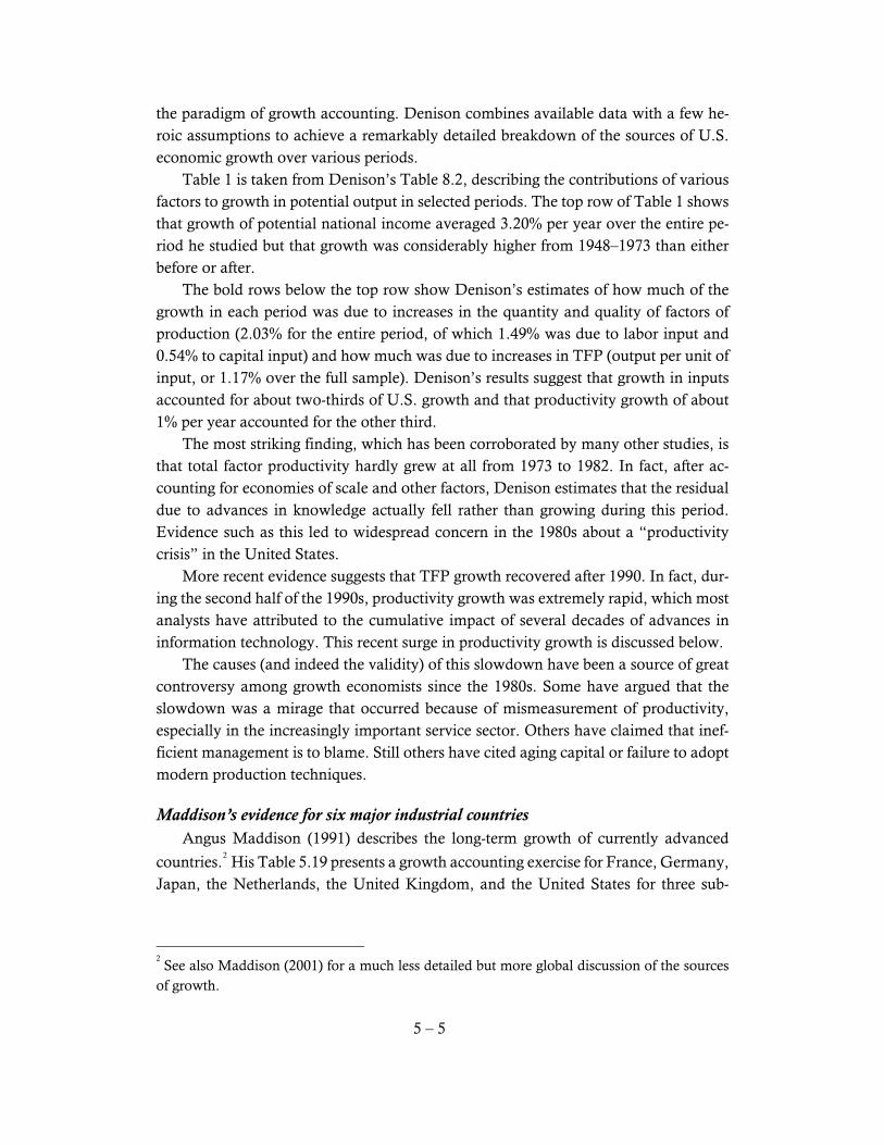
The estimate of total-factor productivity growth will depend crucially on how the au-thor of the study answers these questions. One cannot simply compare results across studies without looking carefully to see the method that the author used in coming up with the measure. Romer gives citations to many of the major authors in the growth accounting lit-erature. In this section, we will survey the results of two major, but dated, works: Ed-ward Denison’s work for the United States and Angus Maddison’s long-term measures for several advanced countries. We then look at a broader sample of countries over the postwar period using the Penn World Tables. Finally, we examine the evidence of Dale Jorgenson and his co-authors about the impact of information technology on U.S. growth in recent decades.

Denison’s estimates for the United States One of the most detailed growth accounting studies of the United States was the life work of Edward Denison of the Brookings Institution, culminating in Denison (1985). Although this work is now very out of date, it is a remarkably clear example of

5 – 5

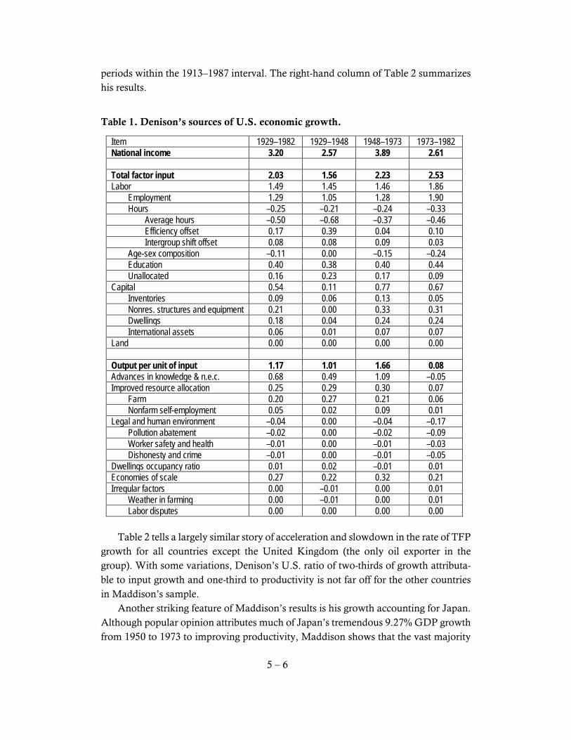
the paradigm of growth accounting. Denison combines available data with a few he-roic assumptions to achieve a remarkably detailed breakdown of the sources of U.S. economic growth over various periods. Table 1 is taken from Denison’s Table 8.2, describing the contributions of various factors to growth in potential output in selected periods. The top row of Table 1 shows that growth of potential national income averaged 3.20% per year over the entire pe-riod he studied but that growth was considerably higher from 1948–1973 than either before or after. The bold rows below the top row show Denison’s estimates of how much of the growth in each period was due to increases in the quantity and quality of factors of production (2.03% for the entire period, of which 1.49% was due to labor input and 0.54% to capital input) and how much was due to increases in TFP (output per unit of input, or 1.17% over the full sample). Denison’s results suggest that growth in inputs accounted for about two-thirds of U.S. growth and that productivity growth of about 1% per year accounted for the other third. The most striking finding, which has been corroborated by many other studies, is that total factor productivity hardly grew at all from 1973 to 1982. In fact, after ac-counting for economies of scale and other factors, Denison estimates that the residual due to advances in knowledge actually fell rather than growing during this period. Evidence such as this led to widespread concern in the 1980s about a “productivity crisis” in the United States. More recent evidence suggests that TFP growth recovered after 1990. In fact, dur-ing the second half of the 1990s, productivity growth was extremely rapid, which most analysts have attributed to the cumulative impact of several decades of advances in information technology. This recent surge in productivity growth is discussed below. The causes (and indeed the validity) of this slowdown have been a source of great controversy among growth economists since the 1980s. Some have argued that the slowdown was a mirage that occurred because of mismeasurement of productivity, especially in the increasingly important service sector. Others have claimed that inef-ficient management is to blame. Still others have cited aging capital or failure to adopt modern production techniques.

Maddison’s evidence for six major industrial countries Angus Maddison (1991) describes the long-term growth of currently advanced

countries.2 His Table 5.19 presents a growth accounting exercise for France, Germany,

Japan, the Netherlands, the United Kingdom, and the United States for three sub-

2 See also Maddison (2001) for a much less detailed but more global discussion of the sources

of growth.

5 – 6

periods within the 1913–1987 interval. The right-hand column of Table 2 summarizes his results.

Table 1. Denison’s sources of U.S. economic growth.

Item 1929–1982 1929–1948 1948–1973 1973–1982 National income 3.20 2.57 3.89 2.61 Total factor input 2.03 1.56 2.23 2.53 Labor 1.49 1.45 1.46 1.86 Employment 1.29 1.05 1.28 1.90 Hours –0.25 –0.21 –0.24 –0.33 Average hours –0.50 –0.68 –0.37 –0.46 Efficiency offset 0.17 0.39 0.04 0.10 Intergroup shift offset 0.08 0.08 0.09 0.03 Age-sex composition –0.11 0.00 –0.15 –0.24 Education 0.40 0.38 0.40 0.44 Unallocated 0.16 0.23 0.17 0.09 Capital 0.54 0.11 0.77 0.67 Inventories 0.09 0.06 0.13 0.05 Nonres. structures and equipment 0.21 0.00 0.33 0.31 Dwellings 0.18 0.04 0.24 0.24 International assets 0.06 0.01 0.07 0.07 Land 0.00 0.00 0.00 0.00 Output per unit of input 1.17 1.01 1.66 0.08 Advances in knowledge & n.e.c. 0.68 0.49 1.09 –0.05 Improved resource allocation 0.25 0.29 0.30 0.07 Farm 0.20 0.27 0.21 0.06 Nonfarm self-employment 0.05 0.02 0.09 0.01 Legal and human environment –0.04 0.00 –0.04 –0.17 Pollution abatement –0.02 0.00 –0.02 –0.09 Worker safety and health –0.01 0.00 –0.01 –0.03 Dishonesty and crime –0.01 0.00 –0.01 –0.05 Dwellings occupancy ratio 0.01 0.02 –0.01 0.01 Economies of scale 0.27 0.22 0.32 0.21 Irregular factors 0.00 –0.01 0.00 0.01 Weather in farming 0.00 –0.01 0.00 0.01 Labor disputes 0.00 0.00 0.00 0.00

Table 2 tells a largely similar story of acceleration and slowdown in the rate of TFP growth for all countries except the United Kingdom (the only oil exporter in the group). With some variations, Denison’s U.S. ratio of two-thirds of growth attributa-ble to input growth and one-third to productivity is not far off for the other countries in Maddison’s sample. Another striking feature of Maddison’s results is his growth accounting for Japan. Although popular opinion attributes much of Japan’s tremendous 9.27% GDP growth from 1950 to 1973 to improving productivity, Maddison shows that the vast majority

5 – 7

of this growth can be explained by increases in factor inputs and with other “ex-plained” sources of growth such as structural changes, technological diffusion, and economies of scale. Japan’s residual (unexplained) TFP growth was considerably lower throughout the sample than France’s or Germany’s. Moreover, Japan’s produc-tivity growth declined after 1973 just as it did in the other countries shown.

Table 2. Maddison’s growth decomposition for six countries.

GDP growth

Augmented factor input contribution

Est. contribu-tions of other

sources

Total explained

growth

Unexplained growth residual

France 1913–1950 1.15 0.48 0.10 0.58 0.57 1950–1973 5.04 2.02 1.17 3.19 1.79 1973–1987 2.16 1.24 0.30 1.54 0.61

Germany 1913–1950 1.28 1.00 0.11 1.11 0.17 1950–1973 5.92 2.42 1.27 3.69 2.14 1973–1987 1.80 0.79 0.50 1.29 0.50

Japan 1913–1950 2.24 1.57 0.53 2.10 0.14 1950–1973 9.27 5.44 2.53 7.97 1.20 1973–1987 3.73 2.95 0.55 3.50 0.23

Netherlands 1913–1950 2.43 2.09 0.22 2.31 0.12 1950–1973 4.74 2.32 1.56 3.88 0.83 1973–1987 1.78 1.30 –0.06 1.24 0.54

United Kingdom 1913–1950 1.29 0.94 0.01 0.95 0.35 1950–1973 3.03 1.76 0.52 2.28 0.73 1973–1987 1.75 0.93 0.08 1.01 0.73

United States 1913–1950 2.79 1.53 0.41 1.94 0.83 1950–1973 3.65 2.54 0.32 2.86 0.77 1973–1987 2.51 2.55 –0.14 2.41 0.10

More comprehensive growth accounting measures The Penn World Tables (PWT) grew out of a research enterprise called the Inter-national Comparison Project, based at the University of Pennsylvania in the 1960s. The latest version of the PWT (Version 9) is described in Feenstra, Inklaar, and

Timmer (2015) and housed at the University of Groningen.3 The goal of the PWT is

to provide internationally comparable figures for GDP and related aggregates with currencies converted at “purchasing-power parity” (PPP) rather than at market ex-change rates. PPP provides a better measure of how much stuff the incomes of people

3 The latest PWT can be downloaded free at http://www.rug.nl/ggdc/productivity/pwt/.

5 – 8

in variables countries can buy in their domestic market, as opposed to how much they would buy, say, in the United States. The latest versions of the PWT have included a collection of growth-accounting

variables: employment, capital input, human capital, labor’s share of GDP (1 – α), and (for many countries) average hours worked. While not nearly as detailed as Denison’s U.S. breakdown, these data facilitate a crude growth accounting exercise for a large

set of countries.4 Table 3 shows growth rates of per-capita GDP and total-factor

productivity for a variety of countries, as reported in the PWT.5 The countries chosen

are those for which data began before 1961, allowing a long sample both before and after 1973.

Table 3. Per-capita GDP and TFP growth

GDP per capita growth TFP growth Europe, US, Canada, Australia, New Zealand

1950-1973

1974-1995

1996-2014

1974-2014

1950-1973

1974-1995

1996-2014

1974-2014

Australia 2.24 1.60 1.79 1.69 -1.62 0.50 0.73 0.61 Austria 4.67 2.19 1.44 1.84 3.06 0.69 0.22 0.47 Belgium 3.57 1.90 1.24 1.59 2.27 0.93 -0.16 0.42 Canada 2.67 1.44 1.49 1.47 1.04 0.01 0.10 0.05 Cyprus 4.58 4.45 0.41 2.58 2.05 1.25 0.06 0.70 Denmark 3.26 1.79 0.85 1.35 1.65 0.99 -0.03 0.52 Finland 4.13 1.83 1.80 1.82 1.70 1.11 0.45 0.81 France 4.15 1.79 1.02 1.44 3.65 1.02 0.25 0.66 Germany 5.24 2.09 1.34 1.75 2.98 1.50 0.50 1.04 Greece 6.06 0.69 0.64 0.67 3.03 -1.08 -0.18 -0.66 Iceland 3.37 1.91 2.10 2.00 1.85 0.47 1.19 0.80 Ireland 2.99 2.76 3.26 2.99 0.43 1.18 1.23 1.20 Italy 4.95 2.31 0.21 1.33 2.80 0.45 -0.78 -0.12 Netherlands 3.76 1.60 1.40 1.50 2.01 0.85 0.35 0.62 New Zealand 2.01 0.84 1.53 1.16 0.85 0.33 0.25 0.29 Norway 3.14 2.92 1.24 2.14 2.21 1.57 -0.09 0.80 Portugal 5.46 2.27 0.95 1.65 3.53 -0.55 -0.15 -0.36 Spain 5.73 1.80 1.20 1.52 3.61 0.84 -0.45 0.24 Sweden 3.06 1.34 1.83 1.57 0.19 0.11 1.10 0.57 Switzerland 3.05 0.65 1.08 0.85 1.07 -0.16 0.41 0.10 Turkey 3.36 2.08 2.50 2.28 3.39 0.09 0.14 0.11 United Kingdom 2.41 1.85 1.54 1.71 0.84 0.96 0.59 0.79 United States 2.55 1.89 1.41 1.67 0.80 0.58 0.92 0.74 4 You worked with these data for one country in your first homework project.

5 Note that the samples vary for some countries because they data may not be available starting

in 1950 or for 2014. All samples begin no later than 1960 and all end no earlier than 2013.

5 – 9

GDP per capita growth TFP growth Latin America and Caribbean

1950-1973

1974-1995

1996-2014

1974-2014

1950-1973

1974-1995

1996-2014

1974-2014

Argentina 1.70 0.02 2.21 1.04 0.56 -0.86 0.25 -0.35 Brazil 4.37 1.50 1.65 1.57 2.91 -0.45 -0.47 -0.46 Chile 1.40 2.72 2.92 2.81 -0.60 0.33 -0.24 0.06 Colombia 2.00 1.97 2.09 2.02 1.48 0.03 0.01 0.02 Costa Rica 3.33 1.23 2.77 1.94 2.69 -1.13 0.41 -0.42 Ecuador 3.06 1.17 1.86 1.49 2.51 -0.70 -0.27 -0.50 Guatemala 1.92 0.42 1.23 0.80 2.06 -0.77 0.22 -0.31 Jamaica 3.82 -0.26 -0.20 -0.23 2.90 -1.28 -0.48 -0.91 Mexico 3.23 0.87 1.50 1.16 2.38 -1.59 -0.51 -1.09 Peru 2.53 -0.61 3.25 1.18 2.27 -2.27 0.03 -1.20 Trinidad and Tobago 4.33 0.06 4.65 2.19 1.84 -1.98 3.27 0.45 Uruguay 0.57 1.91 2.71 2.28 -2.74 -0.26 1.34 0.48 Venezuela 2.44 -0.23 0.47 0.10 1.02 -1.79 -0.81 -1.33

GDP per capita growth TFP growth

Asia 1950-1973

1974-1995

1996-2014

1974-2014

1950-1973

1974-1995

1996-2014

1974-2014

China 1.92 4.69 6.80 5.67 -0.59 1.02 1.95 1.45 China, Hong Kong SAR 6.17 4.96 2.55 3.84 2.67 1.54 0.46 1.04 India 1.60 2.69 5.11 3.81 1.59 0.94 1.44 1.17 Indonesia 2.06 4.68 2.72 3.77 1.44 0.20 -0.14 0.04 Iran 4.57 -2.83 2.16 -0.51 0.54 -4.83 -0.46 -2.80 Israel 5.00 1.84 1.68 1.77 2.86 -0.02 0.41 0.18 Japan 7.45 2.79 0.67 1.81 3.35 -0.70 0.04 -0.36 Jordan 0.83 1.35 1.78 1.55 0.06 -2.11 0.26 -1.02 Malaysia 4.15 4.33 2.78 3.61 2.98 -0.24 0.16 -0.05 Philippines 2.63 0.35 2.74 1.45 0.65 -1.63 0.38 -0.70 Republic of Korea 4.19 7.42 3.71 5.70 1.67 1.58 1.21 1.41 Singapore 7.17 5.52 2.87 4.30 2.10 0.46 -0.23 0.14 Sri Lanka 1.62 3.24 4.80 3.96 0.62 1.01 2.38 1.65 Taiwan 5.75 6.38 3.77 5.17 3.69 1.05 1.11 1.08 Thailand 3.33 5.66 2.47 4.18 1.50 0.53 0.35 0.45

GDP per capita growth TFP growth

Africa 1950-1973

1974-1995

1996-2014

1974-2014

1950-1973

1974-1995

1996-2014

1974-2014

Egypt 2.32 4.33 2.41 3.44 2.72 0.53 -1.17 -0.26 Kenya 0.59 0.30 1.30 0.77 1.14 0.25 -0.51 -0.10 Morocco 1.95 1.64 3.14 2.33 2.61 -0.66 -0.87 -0.76 Nigeria 1.77 -0.15 3.61 1.59 -2.52 -2.72 1.35 -0.83 Senegal -1.61 -0.41 1.32 0.39 0.74 0.08 0.11 0.09 South Africa 2.19 -0.49 1.60 0.48 1.47 -0.75 -0.25 -0.52 Tanzania 2.23 -0.01 2.92 1.35 1.08 0.24 1.27 0.72 Tunisia 4.78 2.15 3.00 2.54 3.38 0.16 0.44 0.29

5 – 10

There are too many countries in Table 3 to summarize all of them in our discussion and each has its own distinct pattern of growth. But there are a few common themes. Many countries show a pattern, similar to that described above, of slower productivity growth after 1973. While productivity growth in the United States recovered strongly after 1995, this was not true in many other wealthy countries. Table 3 shows the strong growth of many East Asian countries, some before and some after 1973. Latin Amer-ica has had a checkered growth record, with many countries experiencing negative productivity growth over long periods.

Information technology and U.S. productivity growth The slow growth of productivity in the late 20th century is particularly surprising because of the rapid advancement in microelectronic technologies. Hardware effi-ciency in computing and telecommunications multiplied rapidly, as reflected in “Moore’s Law,” an observation by Intel co-founder Gordon Moore that microproces-sor speed seemed to double about every 18 months. Yet despite this rapid advance in a key and pervasive technology, overall productivity growth grew only slowly through the 1970s and 1980s. Robert Solow once quipped that “computers are everywhere, except in the productivity statistics.” However, historians of technology have always known that new technologies of-ten require years or decades to develop complementary technologies that allow them

to have a wide-spread positive effect on productivity.6 Electricity could not have a ma-

jor economic effect until power grids were in place and efficient electric light bulbs and motors were affordable. The laser was invented in 1958 but had little economic impact until it was incorporated in measuring, cutting, communication, and printing technol-ogies twenty years later. True to form, productivity began to surge in the 1990s and there is considerable evidence that advances in information technology (IT) are the main reason. Indeed, in a popular book, journalist Thomas Friedman (2005) argues that we have only seen the very beginnings of the productivity effects of the conver-gence of modern information technologies. Reed alumnus Dale Jorgenson has done extensive research on identifying the im-pact of information and communication technologies (ICT) on growth in the U.S. and other countries. A well-known (but now dated) example is his presidential address to the American Economic Association, Jorgenson (2001). A more recent analysis is Jorgenson and Vu (2016). Figure 1 (Figure 2 from their paper) shows their estimates of the contributions to world economic growth of (starting from the bottom of their bar graphs) hours worked, labor quality (human capital), non-IT capital, IT capital, and TFP over four time peri-ods between 1990 and 2012.

6 See, for example, Mokyr (1990) and the essays in Rosenberg (1982).

5 – 11

Figure 1. Jorgenson and Vu's estimates for world economic growth

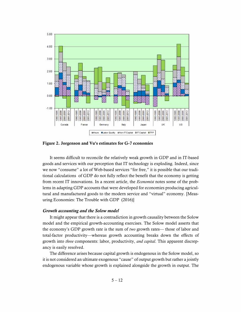
For individual G-7 economies, they provide the breakdown shown in Figure 2 (which is Figure 4 in their paper). The relatively large contribution of IT capital in the United States, United Kingdom, and Canada is not surprising, since these countries are widely recognized as being “early adopters” and leading the IT revolution. Indeed, looking at the depressed (by the financial crisis) 1% U.S. growth rate from 2005–12, almost half of this growth is attributed to IT capital. Another striking feature of Figure 2 is how common negative TFP growth has been among these countries in this century. Italy and Canada have had negative esti-mated TFP growth in both periods since 2000, while the UK and France have slid into negative numbers since 2005. Contrast this performance with Japan, which moved from negative TFP growth through the 1990s to strong positive growth after 2000 and Germany, which has had strong positive TFP growth through the sample period.

5 – 12

Figure 2. Jorgenson and Vu's estimates for G-7 economies

It seems difficult to reconcile the relatively weak growth in GDP and in IT-based goods and services with our perception that IT technology is exploding. Indeed, since we now “consume” a lot of Web-based services “for free,” it is possible that our tradi-tional calculations of GDP do not fully reflect the benefit that the economy is getting from recent IT innovations. In a recent article, the Economist notes some of the prob-lems in adapting GDP accounts that were developed for economies producing agricul-tural and manufactured goods to the modern service and “virtual” economy. [Meas-uring Economies: The Trouble with GDP (2016)]

Growth accounting and the Solow model It might appear that there is a contradiction in growth causality between the Solow model and the empirical growth-accounting exercises. The Solow model asserts that the economy’s GDP growth rate is the sum of two growth rates— those of labor and total-factor productivity—whereas growth accounting breaks down the effects of growth into three components: labor, productivity, and capital. This apparent discrep-ancy is easily resolved. The difference arises because capital growth is endogenous in the Solow model, so it is not considered an ultimate exogenous “cause” of output growth but rather a jointly endogenous variable whose growth is explained alongside the growth in output. The

5 – 13

Solow model explains both output and capital growth in terms of exogenous increases in labor input and productivity. If capital were to stop growing in the Solow model, then output growth at rate n + g could not be sustained, so growth in capital input is surely an ongoing contributor to Solovian growth. In contrast, growth accountants treat inputs of both capital and labor as essentially exogenous factors, so output growth is divided three ways. Neither way of thinking of growth is wrong, they are just differ-ent approaches that hold a different set of factors constant. To see more clearly the connection between growth accounting and the Solow model, consider an economy that is growing along a Solovian steady-state balanced-growth path with the labor force growing at 2% and Harrod-neutral productivity

growth of 1% (i.e., n = 0.02 and g = 0.01), and with an output-capital elasticity αK of

0.3 output-labor elasticity αL of 0.7. GDP and the capital stock in this economy would

grow at 3% in the steady state. Growth accountants would attribute ( )/K K Kα = 0.3

× 3% = 0.9% of this to capital growth, ( )/L L Lα = 0.7 × 2% = 1.4% to labor growth,

and the remaining 0.7% to growth in total factor productivity.

Why does growth accounting seem to undervalue the impact of /A A , reducing its measured effect on GDP growth from 1.0% to 0.7%? The answer lies in the discus-sion above of what is held constant in each case. Recall that Harrod-neutral technical progress of the kind used in the Solow model brackets the technology term in with labor input in the production function. For example, a Cobb-Douglas production for the economy in our example would be written

( )0.70.3 .Y K AL= (1)

The direct effect of a 1% increase in A in equation (1) is a 0.7% increase in Y. This is what growth accounting measures. However, we know that on a Solow balanced-growth path, the increase of 1% in A would lead to a 1% increase in K, which would in turn increase Y by an additional 0.3%. Thus, the direct impact of productivity growth is only 0.7% per year, but if that increase induces an additional increase in the capital stock (as is the case on a Solow balanced-growth path), there would be an ad-ditional indirect effect that would lead to a full 1% increase in GDP.

5 – 14

C. The Convergence Question

While growth accounting can be performed on individual economies without mak-ing international comparisons of income or growth, some of the important implica-tions of the Solow model, such as convergence, require comparable data for a cross section of economies. The late Irving Kravis along with Alan Heston, Robert Sum-mers, and other economists based at the University of Pennsylvania, devoted several decades to the development of an international database in which major economic aggregates were measured on a comparable basis using purchasing-power parity rather

than exchange rates to convert among currencies.7 In the early 1990s, their Penn

World Table (PWT) became the standard data set for international comparisons of growth rates. The PWT enabled economists to try a new approach to testing the implications of the Solow growth model. If growth rates, income levels, investment rates, and other macroeconomic variables can be compared across countries, then it is possible to per-form a cross-sectional study of how growth rates or income levels are affected by the characteristics of economies. A voluminous literature continues to grow examining the determinants of growth across countries, testing for the effects of everything from climate to political stability to religion. One important implication of the Solow model that has been examined repeatedly in this literature is convergence. As Romer discusses in detail, the Solow model implies that the per-capita income levels of countries with similar production functions, saving rates, and growth rates of population and technology will converge over time to the same level. This implies that countries that have low initial levels of income should, other things being equal, grow more rapidly than richer countries, allowing them grad-ually to close the income gap. Romer’s equation (1.36) on page 33 expresses the growth rate as a function of the level of initial per capita income. The left-hand side is the country’s rate of growth over a period (from 1870 to 1979, in this case), while the expression after b on the right is the log of its level of per-capita income at the beginning of that period. Equation (1.36) expresses the left-hand or dependent variable as a linear function of the right-hand or independent variable. The line expressing the functional relationship has a slope of b and intercepts the vertical axis at a. If b < 0, then the line slopes downward and richer countries grow more slowly than poorer ones, so some

7 Purchasing power parities are conversion rates between currencies at which the currencies

will buy equivalent amounts of some market basket of goods in their respective countries.

5 – 15

degree of convergence occurs.8 This b coefficient is closely related to the speed of con-

vergence represented by λ in Romer’s “speed of convergence” discussion on pages 25 and 26. If the growth rate on the left-hand side is expressed in percent per year (as is

usual), then –b = λ.

Graphical evidence on convergence The simplest way to examine the convergence question is just to plot growth rates of countries against their initial levels of per-capita income. Romer’s Figures 1.7, 1.8, and 1.9 on pages 33–36 show such plots for several groups of countries. In Figure 1.7, covering a sample of currently industrial countries using data from 1870–1979, a neg-ative relationship is apparent. This is less true in Figure 1.8, where other countries that were at comparable levels of income in 1870 are added. The evidence is especially chaotic in Figure 1.9, which includes most countries of the non-Communist world over the 1960–89 period. It is difficult to discern visually any evidence of a downward-sloping relationship between initial income and growth in Figure 1.9 and, in fact, the best-fit regression line in such samples sometimes slopes slightly upward. Although it is very useful in gaining an appreciation for the overall patterns in the data, the visual method of analysis cannot answer specific questions about the slope of the best-fit relationship between the variables. It is also difficult to extend the visual framework to more than one explanatory variable. In order to be more precise about the statistical relationship between the variables, we use the method of linear regression analysis to estimate a best-fit line using the data points of a scatter plot such as Figures 1.7 through 1.9. Before examining the growth data further, we digress to consider how this method works.

A digression on the econometrics of linear regression To use data on many countries to estimate the value of b and to test whether it is negative, we use a statistical technique called linear regression. The basic idea of linear regression is to fit a straight line to the collection of data points that we observe for our two variables. For simplicity of exposition, let the independent variable be called x and the dependent variable y. Using notation similar to Romer’s, the linear relationship between the variables can then be written yi = a + bxi, where i is an index that ranges over all the countries in the sample. Finding the best-fit line amounts to estimating the values of the unknown parameters a and b. We now digress at some length to introduce the concept of linear regression as a method of estimating the parameters of economic

8 This concept of convergence is often called β-convergence. A related concept, σ-convergence,

examines whether the cross-sectional variance of per-capita income among countries or regions declines over time.

5 – 16

relationships. After this digression we shall return to the examination of some regres-sions involving economic growth rates and tests of the convergence hypothesis.

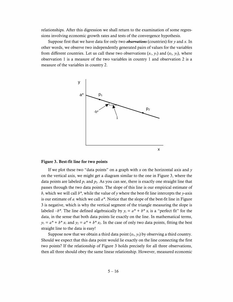
Suppose first that we have data for only two observations (countries) for y and x. In other words, we observe two independently generated pairs of values for the variables from different countries. Let us call these two observations (x1, y1) and (x2, y2), where observation 1 is a measure of the two variables in country 1 and observation 2 is a measure of the variables in country 2.

a*

-b* 1

p2

p1

x

y

Figure 3. Best-fit line for two points

If we plot these two “data points” on a graph with x on the horizontal axis and y on the vertical axis, we might get a diagram similar to the one in Figure 3, where the data points are labeled p1 and p2. As you can see, there is exactly one straight line that passes through the two data points. The slope of this line is our empirical estimate of b, which we will call b*, while the value of y where the best-fit line intercepts the y-axis is our estimate of a, which we call a*. Notice that the slope of the best-fit line in Figure 3 is negative, which is why the vertical segment of the triangle measuring the slope is labeled –b*. The line defined algebraically by yt = a* + b* xt is a “perfect fit” for the data, in the sense that both data points lie exactly on the line. In mathematical terms, y1 = a* + b* x1 and y2 = a* + b* x2. In the case of only two data points, fitting the best straight line to the data is easy!

Suppose now that we obtain a third data point (x3, y3) by observing a third country. Should we expect that this data point would lie exactly on the line connecting the first two points? If the relationship of Figure 3 holds precisely for all three observations, then all three should obey the same linear relationship. However, measured economic

5 – 17

relationships are never that precise. Variables are observed with error and the relation-ship between any two variables is usually subject to disturbances by additional varia-bles that are not included in the equation (and often by variables whose values cannot be observed at all). Consequently, econometricians usually interpret the hypothesis of a linear relationship to assert that all of the data points should lie close to a straight line. It would be very unusual for the added data point to lie exactly on the line that passed through the first two.

In order to allow for this “imperfection” in our two-variable linear relationship, we add a disturbance term or error term to the equation. The resulting equation looks like

,i i iy a bx= + + ε

where εt is the disturbance term, which is usually modeled as a random variable whose

value for each observation are assumed to be drawn from a given probability distribu-tion.

p3

p2

p1

x

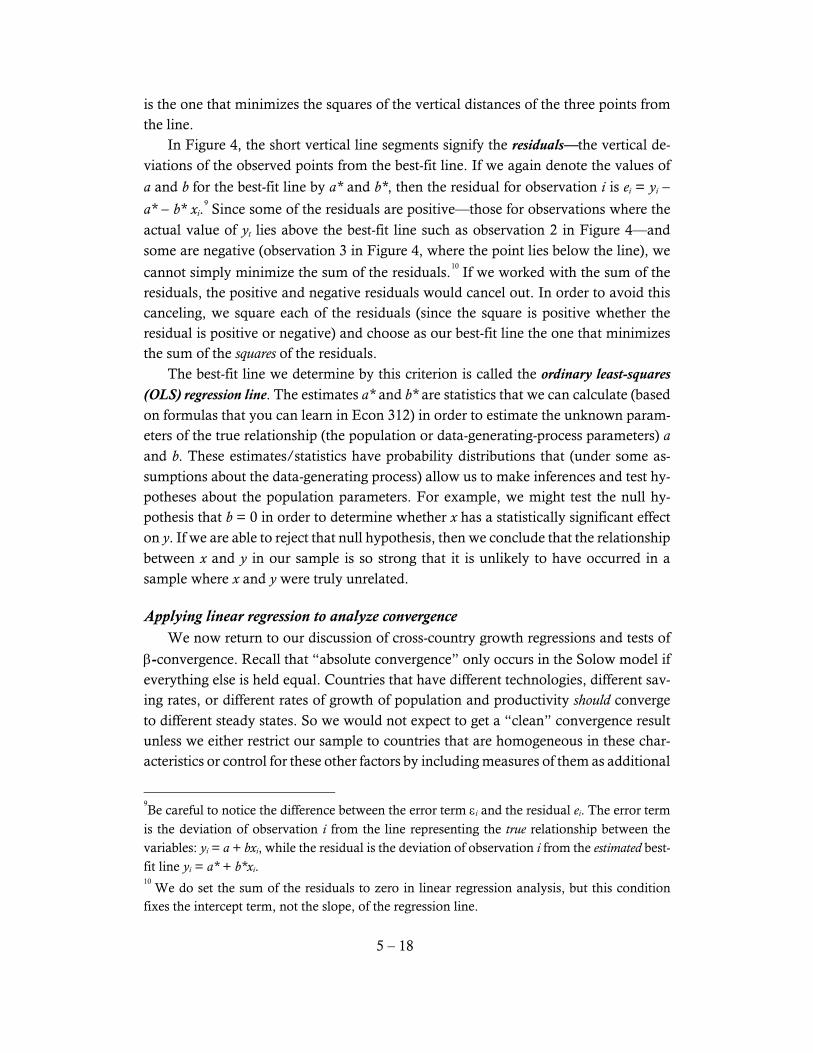
y Length of this segment is the residual e2

Figure 4. Best-fit line with three points

Suppose that the three data points are as shown in Figure 4, so that they do not line up on the same straight line. Now there is no single line that fits all three data points exactly. What criterion should we use to select which line best fits the three data points? In order to answer that question, we must first choose a method to measure “how close” any particular line lies to the collection of three points, and then find and choose the line that lies “closest” to the points according to that measure. The measure most often chosen is that of least-squares, and the line that is chosen as the best-fit line

5 – 18

is the one that minimizes the squares of the vertical distances of the three points from the line.

In Figure 4, the short vertical line segments signify the residuals—the vertical de-viations of the observed points from the best-fit line. If we again denote the values of

a and b for the best-fit line by a* and b*, then the residual for observation i is ei = yi −

a* − b* xi.9 Since some of the residuals are positive—those for observations where the

actual value of yt lies above the best-fit line such as observation 2 in Figure 4—and some are negative (observation 3 in Figure 4, where the point lies below the line), we

cannot simply minimize the sum of the residuals.10

If we worked with the sum of the residuals, the positive and negative residuals would cancel out. In order to avoid this canceling, we square each of the residuals (since the square is positive whether the residual is positive or negative) and choose as our best-fit line the one that minimizes the sum of the squares of the residuals.

The best-fit line we determine by this criterion is called the ordinary least-squares (OLS) regression line. The estimates a* and b* are statistics that we can calculate (based on formulas that you can learn in Econ 312) in order to estimate the unknown param-eters of the true relationship (the population or data-generating-process parameters) a and b. These estimates/statistics have probability distributions that (under some as-sumptions about the data-generating process) allow us to make inferences and test hy-potheses about the population parameters. For example, we might test the null hy-pothesis that b = 0 in order to determine whether x has a statistically significant effect on y. If we are able to reject that null hypothesis, then we conclude that the relationship between x and y in our sample is so strong that it is unlikely to have occurred in a sample where x and y were truly unrelated.

Applying linear regression to analyze convergence We now return to our discussion of cross-country growth regressions and tests of

β-convergence. Recall that “absolute convergence” only occurs in the Solow model if everything else is held equal. Countries that have different technologies, different sav-ing rates, or different rates of growth of population and productivity should converge to different steady states. So we would not expect to get a “clean” convergence result unless we either restrict our sample to countries that are homogeneous in these char-acteristics or control for these other factors by including measures of them as additional

9Be careful to notice the difference between the error term εi and the residual ei. The error term

is the deviation of observation i from the line representing the true relationship between the variables: yi = a + bxi, while the residual is the deviation of observation i from the estimated best-fit line yi = a* + b*xi. 10

We do set the sum of the residuals to zero in linear regression analysis, but this condition fixes the intercept term, not the slope, of the regression line.

5 – 19

explanatory variables in the regression equation (i.e., test “conditional convergence”). Both of these strategies have been followed in a large empirical literature examining convergence. In the next two sections, we consider first a few studies that have tried to use homogeneous economies to examine absolute convergence, then we look at studies of “conditional convergence” that correct for differences in steady states among countries. The basis for regression analyses of convergence lies in the off-the-balanced-growth-path properties of the Solow model. In equation (1.29) on page 25, Romer shows that the convergence process of a Solow economy can be approximated as

( ) ( ) * ,k t k t k≅ −λ − or

( )( ) ( )

*1 .

k t kk t k t

= −λ −

(2)

If the production function is Cobb-Douglas with constant returns to scale and capital

elasticity α, then

( )( )

( )( ) ( ) ( )

1

* *1 1 .

y t k t k yy t k t k t y t

α

= α = −λα − = −λα −

Applying the standard formulas for growth rates of products, total output should grow at rate

( )( )

( )( )

( )( )

( )( ) ( )

1

*1

Y t y t A t L t yg n

Y t y t A t L t y t

α

= + + = −λα − + +

and per-capita output should grow at rate

( )( )

( )( ) ( )

1

*1 .

Y t L t yg

Y t L t y t

α

− = −λα − +

(3)

Equation (3) shows that per-capita GDP growth in a Solow economy depends on three factors: (1) the steady-state growth rate g, (2) the steady-state level of y*, and (3) the current level of y(t). If the economies in the sample can be assumed to be converg-ing to the same steady-state growth path, then y* and g will be the same and the only factor affecting growth should be the initial level of income y(t). This leads to a regres-sion specification similar to Romer’s equation (1.36).

5 – 20

Regression studies of absolute convergence across countries What set of economies can we reasonably assume to converge to the same steady-state growth path? Barriers to capital and technology mobility and international differ-ences in saving behavior and legal environments could make such an assumption un-reasonable for highly diverse samples of countries. In this section and the next, we examine two sets of studies that have tested absolute convergence. First, we discuss the evidence of an early study of advanced industrial countries by William Baumol (1986) and a follow-up study by Bradford De Long (1988). In the next section, we consider a series of studies by Robert Barro and Xavier Sala-i-Martin that examines absolute convergence among sub-national regions among which many of these differ-ences may be less important. Romer equation (1.37) presents Baumol’s OLS best-fit line for the regression equa-tion described in (1.36). As you can see, Baumol’s estimate of b is negative and very close to –1. This suggests strong confirmation of the convergence hypothesis. Since both the dependent and independent variables are expressed in logs, the coefficient b has the dimension of an elasticity. Recall that when the log of a variable changes by 0.01, this is approximately equivalent to a 1% change in the variable’s level because when the log of the variable increases by 0.01, the level of the variable increases by a

factor of e0.01 ≈ 1.01. Thus, Baumol’s results suggest that a 1% higher level of a coun-

try’s income in 1870 is associated with a 1% smaller amount of growth between 1870

and 1979, implying near perfect convergence.11

Before we accept an estimate such as Baumol’s estimated b, we should worry about how likely it is that this negative estimate could have resulted just from random varia-tion in a sample where there was no true relationship between the dependent and in-dependent variables. For example, we would not be too surprised to find a negatively sloped regression line for a sample of only two or three countries even if there was no true negative relationship. Even with sixteen countries, we might be quite skeptical of the evidence for a negative relationship if the scatter of points did not conform closely to the estimated line—in other words, if the residuals were very large in absolute value. We can quantify the confidence that we may place in an estimate such as Baumol’s by performing a statistical test of the hypothesis that b = 0. We can feel more confident that convergence actually occurs if we are able to reject, at a chosen level of signifi-cance, the hypothesis that this result would occur with random sampling from a true data-generating process in which there was no relationship (i.e., one in which b = 0). The number (0.094) that is shown in parentheses below the estimated slope coeffi-cient in Romer’s equation (1.37) is called the standard error of the estimated coefficient.

11

In terms of the λ parameter we have used in earlier discussions of convergence, Baumol’s estimate of 0.995 implies that 99.5% of the initial income differentials were eliminated in one “period,” which in this case is 109 years.

5 – 21

It is an estimate of the standard deviation of the coefficient estimate. To test the hy-pothesis that b = 0, we divide the coefficient value by its standard error. The quotient

that results (−10.6) is referred to as the t-statistic of the coefficient. Although the exact

critical value for choosing whether to accept or reject the null hypothesis of a zero coefficient depends on the level of significance that you choose and on the size of the sample, a common rule of thumb is that you can usually reject the hypothesis of no relationship between the variables with 95% confidence if the t-statistic exceeds 2 in absolute value. Since the absolute value of Baumol’s coefficient is greater than 10, it

seems extremely unlikely that his β-convergence result occurred due to random varia-tion. This is confirmed by the scatter diagram shown in Romer’s Figure 1.7, which shows that the sample conforms very closely to a downward-sloping regression line. On the line below the regression equation on page 33, Romer reports the R2 statis-tic for the regression. The R2 measures the overall goodness of fit of the regression. It is the share of the variation in the dependent variable (growth) that is explained by vari-ation in the independent variable (initial income level). Thus, in Baumol’s regression, the variations in the initial level of per capita income explain 87% of the variation across the sample of countries in growth rates. However, Baumol’s evidence in favor of convergence may not be as convincing as a first reading would suggest. The argument made by Bradford De Long in criticism of Baumol’s paper (described by Romer beginning on page 34) illustrates one of the pitfalls of econometrics. De Long argues that Baumol’s sample was not randomly drawn, but rather included precisely the small group of countries of the world that had converged. Thus, De Long claims that Baumol had (unintentionally) stacked the deck

in favor of finding convergence through his choice of sample countries.12

As you can see from Romer’s Figures 1.8 and 1.9, the case for convergence is much weaker for larger groups of countries, casting doubt on the generality of Baumol’s result. Baumol and De Long wrote the preamble for what has become a voluminous lit-erature using cross-country growth regressions to evaluate convergence. Much of the subsequent work has tested conditional rather than absolute convergence, including variables in the regression to account for differences among countries that might lead them to different steady-state growth paths. Before we examine these conditional-con-vergence studies, we consider a second set of studies of absolute convergence.

Tests of absolute β-convergence using sub-national data Absolute convergence is plausible only when it is reasonable to assume that the economies in the sample share the same parameters. This may be more reasonable among sub-national regions within a relatively homogeneous country or area than

12

Baumol’s choice of countries was natural: he chose the countries for which good macroeco-nomic data were available, which, for obvious reasons, were the richest countries.

5 – 22

across broader samples. Robert Barro and Xavier Sala-i-Martin performed absolute convergence studies for three kinds of sub-national samples: U.S. states, Japanese pre-fectures, and regions within the European Union (Barro and Sala-i-Martin (1991) and Barro and Sala-i-Martin (1992)). They summarize their results in Chapter 11 of their growth text, Barro and Sala-i-Martin (2004), from which the following figures are drawn.

Figure 5. Growth and initial income of 47 states

Figure 5 shows a diagram similar to Romer’s Figures 1.7, 1.8, and 1.9 for 47 states.

13 The vertical axis is the annual growth rate of personal income per person from 1880

to 1990. The horizontal axis measures 1880 income. The close negative association shown in Figure 5 leads us to expect a strongly negative estimate for b in a correspond-ing regression equation. Indeed, Barro and Sala-i-Martin’s basic regression yields an

estimated coefficient of −0.0174 with a standard error of 0.0026, so the t-statistic of –

6.7 is larger than 2 in absolute value and allows us to reject the hypothesis that this association occurred due to random chance. These results are relatively robust to

13

Reproduced from Figure 11.2 of Barro and Sala-i-Martin’s Economic Growth. Oklahoma, Alaska, and Hawaii are excluded because they were not states in 1880.

5 – 23

changes in the time period and to the separation of the sample into Midwest, South,

East, and West regions.14

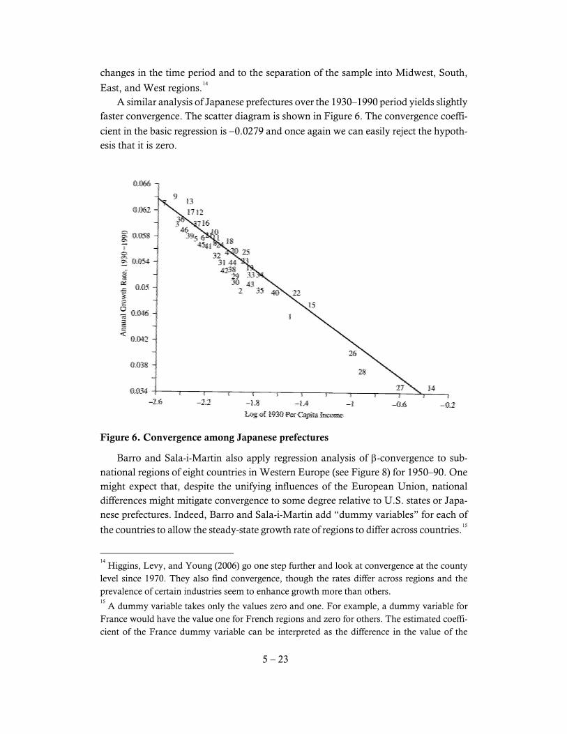
A similar analysis of Japanese prefectures over the 1930–1990 period yields slightly faster convergence. The scatter diagram is shown in Figure 6. The convergence coeffi-

cient in the basic regression is −0.0279 and once again we can easily reject the hypoth-esis that it is zero.

Figure 6. Convergence among Japanese prefectures

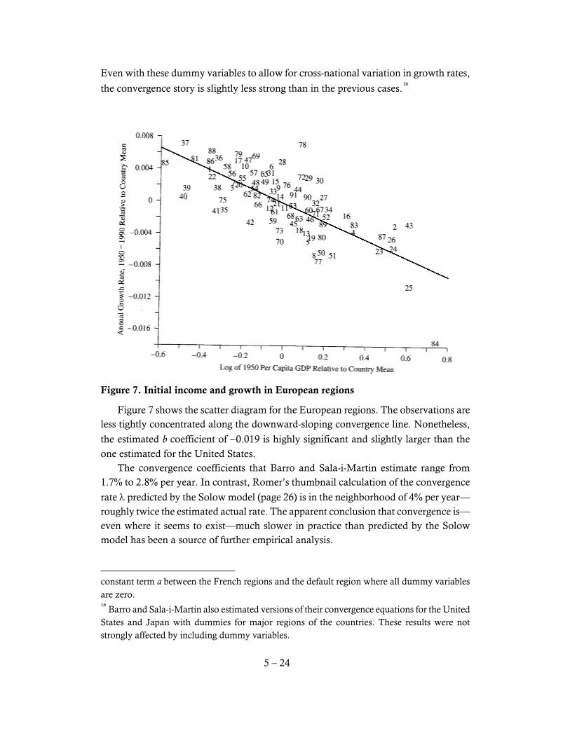
Barro and Sala-i-Martin also apply regression analysis of β-convergence to sub-national regions of eight countries in Western Europe (see Figure 8) for 1950–90. One might expect that, despite the unifying influences of the European Union, national differences might mitigate convergence to some degree relative to U.S. states or Japa-nese prefectures. Indeed, Barro and Sala-i-Martin add “dummy variables” for each of

the countries to allow the steady-state growth rate of regions to differ across countries.15

14

Higgins, Levy, and Young (2006) go one step further and look at convergence at the county level since 1970. They also find convergence, though the rates differ across regions and the prevalence of certain industries seem to enhance growth more than others. 15

A dummy variable takes only the values zero and one. For example, a dummy variable for France would have the value one for French regions and zero for others. The estimated coeffi-cient of the France dummy variable can be interpreted as the difference in the value of the

5 – 24

Even with these dummy variables to allow for cross-national variation in growth rates,

the convergence story is slightly less strong than in the previous cases.16

Figure 7. Initial income and growth in European regions

Figure 7 shows the scatter diagram for the European regions. The observations are less tightly concentrated along the downward-sloping convergence line. Nonetheless,

the estimated b coefficient of −0.019 is highly significant and slightly larger than the

one estimated for the United States. The convergence coefficients that Barro and Sala-i-Martin estimate range from 1.7% to 2.8% per year. In contrast, Romer’s thumbnail calculation of the convergence

rate λ predicted by the Solow model (page 26) is in the neighborhood of 4% per year—roughly twice the estimated actual rate. The apparent conclusion that convergence is—even where it seems to exist—much slower in practice than predicted by the Solow model has been a source of further empirical analysis.

constant term a between the French regions and the default region where all dummy variables are zero. 16

Barro and Sala-i-Martin also estimated versions of their convergence equations for the United States and Japan with dummies for major regions of the countries. These results were not strongly affected by including dummy variables.

5 – 25

Figure 8. Regions used in European convergence studies

Note that one of the crucial determinants of the convergence rate in the Solow

model is α, the share of capital in GDP. If we consider capital to be the traditional, plant and equipment measure, then capital’s share is around 1/3. However, Mankiw, Romer, and Weil (1992) (see below) demonstrate that including returns to human cap-ital in the measure of capital’s share raises the ratio to about 2/3, which in turn cuts the predicted rate of convergence in half—making it much closer to the rates estimated by Barro and others. The Mankiw, Romer, and Weil explanation of the apparently slow rate of convergence has been highly influential, though somewhat controversial.

5 – 26

Testing conditional β-convergence Although it is plausible that conditions and behavior are sufficiently similar across states, prefectures, and regions within Western Europe that we might expect that they would converge to a common steady-state growth path, it seems unlikely that the same homogeneity applies across all countries of the world. For example, Romer’s Figure 1.9 reveals little evidence of negative correlation between initial income and growth

across a large sample of countries.17

Convergence tests among less homogeneous econ-omies usually add other “control” variables in the growth regression alongside initial per-capita income. Including the other variables that affect the steady-state growth rate allows the effect of initial income to be examined even when steady-state growth rates differ. To see how a conditional-convergence regression might work, consider four coun-tries that obey the Solow growth model. The countries differ in two ways: two have a high saving rate and two have low saving rates. Two have relatively low initial endow-ments of capital per worker and two have relatively high initial capital. Call these countries HSLK, HSHK, LSLK, and LSHK, respectively, according to the definitions in Table 5. We assume that all other aspects of the countries (production function, level and rate of technological progress, population growth rate) are identical.

Table 4. Definitions of four example countries

Initial Capital/Worker

Low High Saving Rate

Low LSLK LSHK High HSLK HSHK

The Solow model tells us that per-capita income in the two countries with high saving rates will converge to a higher balanced-growth path than those with low saving rates. The initial level of per-capita income depends only on capital per worker, so the two LK countries begin at low per-capita income and the HK countries start out higher. Figure 8 shows the convergence paths of the four countries to their respective balanced-growth paths. Notice that the most rapid growth over the t0 to t1 time interval occurs in HSLK. Its high saving rate means that this country will move to the higher steady state, while its low initial capital implies that it starts from a lower level. LSHK has the lowest growth rate from t0 to t1 because it starts from high per-capita income and moves to the lower path due to its low saving rate. HSHK and LSLK have similar, intermediate rates of growth, despite their large differences in initial income.

17

For a non-regression approach that demonstrates the implausibility of convergence among the broad sample of countries, see the discussion of Pritchett (1997) in the next section.

5 – 27

Time

Log of per-capita GDP

LSLK

HSLK

HSHK

LSHK

t0

t1

Figure 9. Conditional convergence of four countries

A conditional-convergence regression would capture the behavior of the countries in Figure 9 with an equation such as

(0) ,i i i ig y s= α +β + γ + ε (4)

with gi representing per-capita income growth in country i, yi(0) is initial per-capita

income in i, si is the saving rate in i, and εi is a disturbance term that picks up other

unmeasured effects on the growth rate. The coefficients α, β, and γ are estimated in the regression.

Figure 9 shows that the Solow model predicts β < 0 (as in the absolute-convergence

regressions) and γ > 0. The highest growth rate is achieved by HSLK, where the high

si multiplied by the positive γ coefficient is added to the low yi(0) value multiplied by

the negative β coefficient to assure high growth. Contrast HSLK with LSHK, where

the low saving rate is multiplied by positive γ and the high initial income is multiplied

by negative β, both of which give a lower growth rate. A vast number of cross-country growth regressions have been performed in the last two decades using various combinations of control variables playing the role of si in

equation (4).18

Prominent among the variables that are often assumed to affect the steady-state path are saving and investment rates, education variables, population growth, government budget variables, measures of openness to trade, and various

18

An extensive compilation of the variables used in various studies in given in Table 2 of Durlauf and Quah (1999). This table (now over ten years out of date) spans five pages!

5 – 28

measures of governmental efficiency such as corruption indexes, frequency of revolu-tions, existence of black markets, or indicators of civil liberties.

Mankiw, Romer, and Weil: Taking Solow seriously In an influential paper, N. Gregory Mankiw, David Romer, and David Weil at-tempted to “take Robert Solow seriously” (Mankiw, Romer, and Weil (1992, 407)). They calculated (as you might in a homework assignment) what the steady-state level of output per person would be in the Solow model with a Cobb-Douglas production function:

1

* .s

yn g

α−α

= + + δ (5)

In log terms, equation (5) implies

( )( ) ( ) ( )ln ln 0 ln ln .

1 1

Y tA gt s n g

L t

α α= + + − + + δ −α −α

(6)

Mankiw, Romer, and Weil collected data on the values of n and Y/L for a large

number of countries and ran a regression based on equation (6), assuming that g + δ =

0.05 for all countries. They found considerable support for the Solow model from the

fact that the coefficients on lns and ln(n + g + δ) seemed to be equal in absolute value

and of opposite sign. However, the implied value of α was around 0.6—much larger than the conventional value of 1/3. Mankiw, Romer, and Weil then estimated an augmented model that included hu-

man capital. The results of this model suggested an α for physical capital of about 0.3

and a corresponding coefficient β on human capital of the same magnitude. Both of these values correspond plausibly to the factor shares of physical and human capital, so the Mankiw, Romer, and Weil model was interpreted as supporting the Solow model’s prediction that cross-country income differences were largely a result of dif-

ferences in the amount of (physical and human) capital they had accumulated.19

Studies of conditional convergence abound in the literature. A few of these are examined in a later section on cross-country correlates of growth.

19

This conclusion was challenged by, among others, Klenow and Rodriguez-Clare (1997), who use more refined measures of human capital investment and arrive at a different conclusion. This paper is discussed below.

5 – 29

D. Non-Regression Approaches to Convergence

The concept of σ-convergence An alternative approach to the analysis of convergence is to examine the cross-sectional variation in per-capita income levels at different points in time. If the degree

of variation, measured by the standard deviation σ, declines over time, then σ-conver-gence is said to occur. If all economies were converging to a common Solow balanced-growth path, then

eventually σ should approach zero. However, there are at least two reasons why we

would not expect to observe σ → 0. First, as discussed above, there are good reasons for believing that some countries’ balanced growth paths may lie above or below oth-ers’. This implies that even after complete convergence there will still be a non-degen-erate distribution of per-capita income levels across countries. Second, a realistic ap-plication of convergence theory must recognize that convergence will be interrupted by shocks that move countries upward or downward relative to their balanced-growth paths. These shocks would generate a base level of cross-country variation even when the effects of initial differences in capital intensity were eliminated through conver-gence. Thus, to interpret changes in measured standard deviation of per-capita incomes over time as a test of convergence, we need to make (at least) two important assump-tions relating to the two issues above. First, we need to assume that the cross-country distribution of steady-state paths does not change over the sample period we examine. If changes (unrelated to Solovian convergence) in the world’s economies caused

growth paths of per-capita income to get closer to one another over time, then σ would decline for reasons other than traditional convergence. Similarly, if paths became more

widely different, σ might not fall even if capital-based convergence were occurring. Second, we need to assume that the shocks pushing countries away from their nat-ural paths do not vary in intensity over the sample. If shocks were less pronounced in

the later years of the sample, we would see σ falling even without Solovian conver-gence, whereas if there were many shocks that varied strongly across countries at the

end of the sample, the resulting rise in σ might offset the effects of whatever Solow-type convergence was happening.

These considerations suggest that testing for σ convergence should, like the tests

of absolute β convergence, restricted to economies that are likely to have a common balanced-growth path and similar shocks. Figure 10 shows that the standard deviation of per-capita income across Japanese prefectures has declined markedly since World

5 – 30

War II, though the shock associated with war preparations increased dispersion con-

siderably between 1930 and 1940.20

Figure 10. σ-convergence across Japanese prefectures

Barro and Sala-i-Martin present evidence for U.S. states that shows a similar pat-tern of declining dispersion in per-capita incomes since 1880. For European regions,

they report separate σ-convergence diagrams for regions within each country, which

also show considerable decline in income dispersion.21

Tests of convergence in the cross-country distribution of incomes Although changes in the standard deviation of income can be a useful measure of convergence, there is much more information in evolution of the cross-country distri-bution of income than can be represented by changes in a single measure. Several au-thors have used advanced statistical methods to examine how the entire distribution

has changed over time.22

By looking at year-to-year changes in the relative cross-country income distribu-tion, these authors have estimated the likelihood that countries in particular parts of the distribution (for example, between the 40th and 50th percentiles) will move upward or downward to other parts of the distribution in the following year. Applying these year-to-year “transition probabilities” repeatedly allows one to estimate the “entropy,” or final steady state, of the distribution.

20

Figure 10 is reproduced from Figure 11.7 of Barro and Sala-i-Martin (1995). 21

See Barro and Sala-i-Martin (1995), Figures 11.4 and 11.9. 22

A summary of this literature can be found in section 5.6 of Durlauf and Quah (1999). Among the papers in this literature are Quah (1993) and Bianchi (1997).

5 – 31

Figure 11, which is taken from Durlauf and Quah (1999), shows a transition sur-face for 15 years of convergence, using data taken from year-to-year transitions of 105 countries over the 1960–88 period. The height of the surface at any point measures the likelihood of moving from the relative income position on the Period t axis to the po-sition on the Period t+15 axis in 15 years. Two features of Figure 11 are noteworthy: the strong ridge along the diagonal and the twin peaks along that ridge. Both are com-mon findings in the literature.

Figure 11. Estimated changes in distribution of world incomes after 15 years of convergence

The prominence of the ridge shows that countries tend to remain in the same part of the relative income distribution over time. Countries at the poorer (richer) end are more likely to still be poor (rich) fifteen years later than to have changed theory posi-tion markedly. The twin-peaked pattern shows a tendency for economies to bunch into two groups, richer and poorer, with countries in the middle tending to either move up or down toward one of the groups. These groupings have been dubbed “convergence

clubs” and have been the subject of theoretical as well as empirical examination.23

The idea of convergence clubs has been used to suggest the possibility of “poverty traps,” in which poorer countries remain stuck in a low-income equilibrium. Graham

23

For example, see Basu and Weil (1998).

5 – 32

and Temple (2006) find evidence consistent with the existence of such poverty traps. Sachs et al. (2004) argue that tropical Africa is stuck in a poverty trap and plead for a “big push” of development assistance to aid these countries in escaping it. However, Kraay and Raddatz (2007) find poverty-trap models to be inconsistent with the data for Africa.

Pritchett’s test of plausibility of absolute convergence Not all tests of convergence rely on elaborate statistical methods. One of the sim-plest, but most convincing, tests of convergence is by Lant Pritchett (1997). He inves-tigates absolute convergence or divergence among nations by a simple backward ex-trapolation procedure. The question he poses is “Given the dispersion in per-capita incomes across countries today and the growth that we can measure in the rich coun-tries since 1870, is it plausible that income differentials were much wider in 1870 and that convergence has occurred since then?” Pritchett uses evidence from the growth accounting studies of Angus Maddison (see section B above) to estimate that per-capita income in the advanced countries has grown at an average rate of about 1.5 percent per year since 1870. We do not know enough about historical income levels in other countries to assess directly whether or not they have grown more rapidly than this. We do however have reasonably good

estimates of their current income levels.24

Pritchett’s method is to extrapolate a com-parable 1.5 percent growth rate backward from the current income levels of poor coun-tries, then to ask whether or not the computed 1870 income levels are plausible. He finds that many currently poor countries would have to have had income levels of $100 per person or below (in today’s terms) in 1870 if they have been growing at 1.5 percent since then. However, he estimates the minimum level of per-capita income that produces sufficient caloric intake to prevent starvation at about $250. Thus, he concludes that today’s income distribution cannot represent “convergence” relative to 1870, because the people in currently poor countries could not have survived if their incomes had started out that low. Perhaps Pritchett’s finding is not surprising, given that we do not see strong evi-dence for absolute convergence in the broad sample of countries even over the shorter,

postwar time period.25

Nonetheless, his simple illustration makes a strong case for fo-cusing attention on non-convergent models or on explaining why countries’ balanced-growth paths differ.

24

Pritchett uses the Penn World Table data discussed above. 25

Recall the evidence of Romer’s Figure 1.9.

5 – 33

E. Cross-Country Correlates of Growth and Income

The availability of detailed cross-country data for many countries in the postwar period in the Penn World Table and for a few countries back into the 19th century from Maddison has spawned a cottage industry running growth regressions. The typical such regression relates growth (or income level) to various economic, political, or so-cial characteristics of the country. Growth regressions of this kind nearly always in-clude a measure of initial per-capita income to capture the convergence effect. The author then adds other variables that he thinks might cause countries’ growth paths to differ and tests whether they have an effect. We examine a few such studies below, beginning in the next section with one of the first studies to examine the effects of human capital on growth. Note that most of these studies are relatively dated. There is additional literature that will be included in future editions of the coursebook.

Barro and Lee’s cross-country evidence on human capital One of the most frequently cited cross-country growth studies is Robert Barro and Jong-Wha Lee’s study, which was among the first to incorporate human capital vari-ables. Barro and Lee (1994) report the results many alternative specifications; we focus here on the simplest. Barro and Lee include the following variables that may affect countries’ steady-state paths:

• Investment/GDP ratio. This is essentially the saving rate, as in (4).

• Government consumption/GDP ratio. Taxes to support government con-sumption reduce income available for private investment and consumption. These taxes are never lump-sum in practice, thus higher taxes are likely to dis-courage work and investment.

• Black-market premium on foreign exchange. This variable proxies for the ex-tent to which governments distort prices away from equilibrium, presumably reducing efficiency.

• Revolutions (successful or unsuccessful) per year. More frequent revolutions are believed to reduce per-capita income by lowering the security of property rights and diverting resources from productive activities into protective and political ones.

• Human-capital variables: Male and female school attainment measure educa-tion; life expectancy measures health status.

5 – 34

One of the major obstacles to studying the macroeconomic effects of human capi-tal is the difficulty of measuring it. International agencies and national governments collect data for many countries on school enrollment. However, this measures the flow of education (investment in human capital), not the stock of educated people (human capital itself). In order to overcome this problem, Barro and Lee developed measures of “educational attainment” by combining data from many sources. Barro and Lee measure educational attainment using the shares of the population at any time that have achieved four levels of schooling: (1) none, (2) at least some primary education, (3) at least some secondary education, and (4) at least some higher education. They use census data to estimate these shares at five-year intervals for over 100 countries. This procedure leaves many missing “cells,” because not all of the coun-tries have reliable census data at each date. However, by combining the relatively sparse available data on the general population’s educational attainment with more regularly available measures of literacy and school enrollment, they are able to create

satisfactory data for 85 countries for 1965–75 and for 95 countries for 1975–85.26

Barro and Lee present their main results in their Table 5. Because all of the 18

regressions in Table 5 tell a consistent story, we shall focus on a single one.27

The de-pendent variable in their regression is the ten-year-average growth rate of real per cap-ita GDP either over 1965–75 or 1975–85. They pool the two time periods together in their sample to get a total of 160 growth observations—85 and 95 for the two periods,

respectively.28

Table 6 shows the estimated coefficients of this regression and their standard er-rors. Remember that we can get a sense of how strongly the data support the hypoth-esis that the coefficient is not zero by dividing the estimated coefficient by the standard error. If the resulting t statistic is larger than two in absolute value, then we can be pretty confident that the variable has a non-zero effect for this sample. The negative coefficient on initial GDP gives strong support for the conditional convergence hypothesis. The convergence rate of 2.55% per year is in the range of estimates that we have seen above for states, prefectures, and regions, and is typical of the larger literature from which this study is drawn. The other non-human-capital variables have the expected signs. Investment is good for growth, which implies that countries with higher saving/investment rates converge to higher balanced-growth paths. Government consumption seems to lower

26

The original paper discussing the human-capital variables is Barro and Lee (1993). An up-dated version of the data, which are available at www.nber.com, is described in Barro and Lee (2000). 27

We present detailed results for column (2) of Barro and Lee’s Table 5. 28

This kind of sample is called panel data and is discussed below.

5 – 35

the growth path, consistent with greater disincentives from higher tax rates. Distorted markets and revolutions are both very bad for growth, as expected.

Table 5. Barro and Lee’s regression results.

Explanatory variable Estimated effect (Standard error)

Log of initial GDP –0.0255 (0.0035)

Investment/GDP 0.077 (0.027)

Government consumption/GDP –0.155 (0.034)

Black-market premium –0.0304 (0.0094)

Revolutions –0.0178 (0.0089)

Male secondary school attainment 0.0138 (0.0042)

Female secondary school attainment –0.0092 (0.0047)

Log of life expectancy 0.0801 (0.0139)

Barro and Lee emphasize the human-capital measures, which were the novelty of this particular paper. Since this is a topic of interest to us as well, we will consider them in more detail. The human-capital coefficients support the idea that male schooling and life expectancy increase growth. However, the coefficient on female secondary school attainment is estimated to be negative and achieves borderline statistical signif-icance. The male schooling variable implies that giving all of the males in the popula-tion another year of high school education at the beginning of the period would raise growth during the 10-year period by 1.4 percentage points. Similarly, an increase in life expectancy of 10 years would increase growth by about 1.3 percentage points, pre-sumably reflecting the productivity advantages of better health and nutrition. The negative estimated coefficient on female school attainment is a puzzle, but one that is repeated consistently throughout their study. Barro and Lee (p. 18) specu-late that “a high spread between male and female secondary attainment is a good measure of backwardness; hence, less female attainment [at the beginning of the pe-riod] signifies more backwardness and accordingly higher growth potential through the convergence mechanism.” However, convergence effects should already be cap-tured in the regression through the presence of the initial per capita GDP variable, so any convergence effects entering through the education variables are presumably of second order.

5 – 36

The estimated coefficient on the male educational attainment variable is larger in absolute value and more statistically significant than the negative female coefficient, so the general view from the Barro and Lee study is that human capital has an overall positive effect on growth. However, we must interpret the results of Barro and Lee’s regression carefully. Should a higher level of education have a growth effect or just a level effect? In the neoclassical model, an increase in the stock of human capital would lead to a higher level of per capita income, but not to a higher steady-state growth rate. Since Barro and Lee’s explanatory variable is the beginning-of-period stock of human capital, not the accumulation of human capital through the period, a positive coefficient implies a growth effect. A higher level of human capital implies a higher growth rate for real out-put. Thus, Barro and Lee’s results seem to suggest support for a model in which higher human capital leads to a higher rate of productivity growth, perhaps because educated workers are better able to adopt new technologies developed in more advanced econ-

omies.29

Robustness in cross-country growth studies Empirical studies of growth rates face a serious econometric problem: the statistics that we use to test whether a variable has a statistically significant effect on growth are based on the assumption that all of the determinants of growth are included on the right-hand side of the regression equation. While a convincing case can be made for the variables that Barro and Lee have included, it is hard to imagine that there aren’t dozens of other variables that affect growth. Indeed, the number of potential growth correlates is limited only by our imagination and the availability of suitable measures. However, it is infeasible to put all of them in a regression equation at the same time. As discussed in an earlier section, we need lots of degrees of freedom for our statistical tests to be able to discriminate effectively between accidental correlations in the data and those that are too strong to have occurred randomly. That means that the number of observations must be much larger than the number of coefficients being estimated in the regression. A cross-country growth regression can have only about 100 country observations, so the number of variables that can be included on the right-hand side must be much lower than 100. Most econometricians would feel uncomfort-able running such a regression with more than about 10 right-hand variables whose coefficients must be estimated.

29

Recall that Mankiw, Romer, and Weil (1992) obtained good econometric results from a con-vergent model with human capital, which suggests level but not growth effects. Recently, Cohen and Soto (2007) have developed a new dataset on international human capital. Their results suggest a growth effect for increased schooling.

5 – 37

Given our limited observations and the plethora of candidate regressors, we are almost certain to leave out something of relevance. This will bias the estimated coeffi-cients of variables that are correlated with the omitted variables. For example, suppose that what really affects growth is the effective enforcement of property rights, but that we do not include a variable measuring this in the equation. We do include a variable indicating whether or not the country has a democratic form of government. Because property rights are more often enforced effectively in democracies, these variables will be correlated. Leaving out the property-right variable will cause the democracy varia-ble to “proxy” for the omitted variable. Because the coefficient on the democracy var-iable will measure both the effects of democracy and those of property rights, it will be a biased measure of the pure democracy effect. If we omit property rights from the equation, our results might suggest that democracy has a significant effect on growth even if it does not. A related problem is that of multicollinearity, which occurs when a set of explana-tory variables is so highly correlated within itself that it is impossible to identify their individual effects. Suppose in the example above that we have measures of both de-mocracy and or property rights, but that all countries that are democratic have good property-rights regimes and all autocratic countries have bad property rights. In this case, democracy and property rights are perfectly correlated (collinear) with one an-other. Our regression may detect that a change from autocracy and bad property rights to democracy and good property rights affects growth, but because we have no obser-vations with democracy and bad property rights or autocracy and good rights, we can-not tell which variable it is that is important. Many sets of variables in growth regres-sions tend to be highly correlated, making it difficult to identify which individual var-iables within these sets are most important. The omitted-variable and multicollinearity problems mean that we must be careful to test the robustness of our results. Variables that seem to affect growth for only a few specifications (collections of right-hand variables) but not for others are termed “frag-ile” while those whose strong effect is consistent for all or most choices of specifica-tions are called “robust.” In an aptly titled paper, Sala-i-Martin (1997) tests the robustness of growth deter-minants by looking at about two million alternative specifications. He assumes that initial per-capita income (the convergence effect) and human capital (life expectancy and education) surely affect growth, so these variables are included in all specifica-tions. He then includes various combinations of 59 additional variables that had been proposed as possible causes of growth differences in the pre-1997 literature. Of these 59, he finds 22 variables to have effects that are robust—statistically significant often enough to suggest that their effects are not due to a fortuitous choice of specifications. He groups the robust variables into the categories shown in Table 7. Some of these variables can be easily interpreted in terms of growth theory. For example, higher rates

5 – 38

of investment correspond to higher saving rates, which should elevate the growth path according to the Solow model. Rule of law should affect income and growth positively because when legal protections are strong, fewer people will choose non-productive activities such as theft and rent-seeking, and because there are fewer thieves, produc-

tive workers will spend less to protect themselves from theft.30

No one should be sur-prised that wars are bad for growth!

Table 6. Variables with robust effect on growth.

Regional variables: Sub-Saharan Africa (−), Latin America (−), Absolute value of latitude (+) Political variables: Rule of law (+), Political rights (+), Civil liberties (+), Revolutions and coups (−), Wars (−) Religious variables: Confucian (+), Buddhist (+), Muslim (+), Protestant (−), Catholic (−) Market distortions and performance: Real-exchange rate distortions (−), Variation in black-market premium (−) Investment: Equipment investment (+), Non-equipment investment (+) Primary-sector production: Primary share in exports (−), Mining share of GDP (+) Openness: Years of openness to trade (+) Economic organization: Degree of capitalism (+) Colonial heritage: Former Spanish colony (−)

Source: Sala-i-Martin (1997). See original paper and those cited therein for variable definitions. However, other variables in Table 7 raise as many questions as they answer. The regional variables verify that growth has been lower than would be expected based on other variables for countries in sub-Saharan Africa, Latin America, and those lying nearer the equator. But these variables do not explain why these countries have had lower growth. To have a true explanation of growth, we need to know what it is about these countries that caused them to grow more slowly. Similarly, the religion and co-lonial heritage variables are probably proxying for characteristics of these societies that are not being measured directly. As economists are able to use more and better measures of social characteristics, an appropriate goal might be the elimination of the significant effects of these dummy variables.

Cross-country vs. panel data estimation The limited number of countries we can observe limits our ability to identify fac-tors that affect growth. One possible method of increasing the number of observations

30

Earlier editions of Romer’s text had a section at the end of Chapter 3 discussing such a model. Interested students may explore this model there.

5 – 39

is to use multiple observations from each country corresponding to different time pe-riods. Datasets with observations that track the same cross-sectional sample over time are called panel data. Using panel data has the advantage of allowing separate historical periods within a country to speak distinctly in the sample. For example, Vietnam, Germany, China, South Africa, Chile, and many other countries have had major changes in the structure of their economies in the last half century. In a purely cross-sectional sample, the growth rate and the values of the independent variables would be averaged over the entire period, ignoring information about changes over time in growth and country characteristics. With panel data, the time periods that these countries were under dif-ferent regimes can be entered as separate observations, potentially increasing the abil-ity of the sample to identify the effects of changes in regimes. However, there are some pitfalls associated with using panel data that often require the use of special econometric techniques. It is likely that many characteristics of a country remain unchanged over time. Those that can be measured (e.g., geography) can be entered into the equation, but those that cannot (e.g., culture) end up contrib-uting to the error term. The desirable statistical properties of the ordinary least squares estimator depend on the assumption that the error term for each observation is an in-dependent draw from a given probability distribution whose value does not depend on any of the other draws. If we have five decadal observations for Mexico and there are unmeasured characteristics of Mexico that contribute in a similar way in each decade, then the five Mexico observations will not be independent. A similar problem occurs with observations from different countries for the same period of time. The oil shock of the 1970s affected all countries of the world at the same time, though perhaps not all in exactly the same way. If, say, France and Belgium were similarly affected by the rise in world oil prices (and if there is no variable in the equation to measure oil-price shocks), then the observations for the 1970s for France and Belgium would likewise not be truly independent. The standard way of compensating for these common country factors and time events is by using a fixed-effects estimation model. This regression equation includes on the right-hand side, in addition to the desired explanatory variables, a dummy

(zero-one) variable for each country and for each time period.31

Any idiosyncratic char-acteristics that affect a country’s growth in all periods are captured in the coefficient of that country’s dummy variable. Any idiosyncratic effects occurring in all countries in

31

For example, a dummy variable for Mexico would have the value one for observations on Mexico and zero for all other observations. Its coefficient then measures (and controls for) any tendency for growth in Mexico to be higher or lower than the world average across all time periods.

5 – 40

a given time period are captured by the coefficient on that time period’s dummy vari-able. What remains to be explained by the coefficients on the explanatory variables are the variations in growth not occurring strictly in one country or time period. Because the coefficients of interest are estimated based on differences across countries of the differ-ences (changes) over time, this estimation model is sometimes called a differences-in-dif-ferences estimator. As noted above, Barro and Lee use a panel-data sample with two observations per country. Because they have so few observations per country, they use an alternative estimation method called a random-effects model that accounts for the correlation be-tween the observations of a single country in the two time periods but does not add a dummy variable for each country. Results from fixed-effects and random-effects mod-els are often, but not always, similar.

Institutions and economic growth A major theme among recent studies of cross-country growth has been attention to the effect of political and social institutions. By “institutions,” economists usually mean man-made characteristics of social and political interaction such as the form of government, the number and kinds of political parties, the size and power of various economic groups (e.g., labor unions and producer organizations), cultural customs, and the effectiveness of law enforcement and judicial systems. Economists hope to explain the differences in growth captured by the regional dummy variables discussed above by careful examination of these institutional characteristics. In Section 4.5, Romer summarizes some institutional growth literature on the effects of geography and colonization on income and growth. An important strain of growth literature has looked at political institutions. Alt-hough Sala-i-Martin (1997) finds five political variables—rule of law, political rights, civil liberties, revolutions and coups, and wars—to be robust predictors of growth in a cross-country sample, some of these are more “outcomes” of policy than “political institutions.” How does one distinguish the effects of political institutions from those of the pol-icies that those institutions promulgate? It is clear from Sala-i-Martin (1997) and the literature that he reviews is that the combination of good institutions and good policies does tend to be associated with high incomes and growth. But if countries with “good institutions” tend to have “good economic policies,” then how can we know if it is the policies or the institutions that correlate with growth? Moreover, if it is institutions

5 – 41

that are relevant, is it good political institutions that lead to high incomes or high in-comes that cause countries to adopt good institutions? Economists and political scien-

tists are still struggling with these problems.32

One related question that has attracted attention from both economists and politi-cal scientists is whether democratic countries tend to grow faster than autocratic ones. Clearly, much will depend on what else is held constant. It may be that democratic institutions affect growth only because democracies tend to enforce the rule of law and protect political rights and civil liberties more effectively and to face a reduced likeli-hood of war or revolution. If the only effect of democracy is through these other vari-ables, then a democracy variable added to an equation that already contains these var-

iables would have no explanatory effect.33

Table 1 of Przeworski and Limongi (1993) summarizes 18 empirical studies by economists and political scientists looking at the effects of democracy on growth in samples from 1950 to the mid-1980s. These authors conclude that the evidence is al-most equally mixed among results favoring democracy and those favoring autocracy, with some studies finding no difference. As noted above, it is likely that policies have a more direct effect on growth than the form of government. Either a democracy or a dictatorship can follow policies that are good for growth or policies that inhibit growth. In terms of policies, economists are broadly in agreement that “economic liberali-zation” policies are likely to enhance growth. Giavazzi and Tabellini (2005) examine the combined effects of democracy and liberalization, taking careful consideration of the order in which changes occur. They use panel data for 1960–2000 for approxi-

mately 135 countries.34

Their measure of economic liberalization is taken from Sachs and Warner (1995), based on the openness of the economy to trade. According to their definition, a country is open in a particular year if none of the following conditions applies:

• average import tariff rate exceeds 40%,

• more than 40% of imports are covered by nontariff barriers,

• the economic system is socialist,

• the black-market premium on the exchange rate exceeds 20%, and

• much of the country’s exports are controlled by the state.

32

See Kurtz and Schrank (2007) for a discussion of the problems of the common measures of political institutions and an analysis suggesting that the causality runs from economic from high incomes to good institutions rather than the other way around. 33

As noted above, the direction(s) of causality are debatable in these equations, so it may be more appropriate to model these political outcomes as dependent variables in their own equa-tions with democracy as one of the explanatory variables. 34

The exact number varies over time depending on the availability of data.

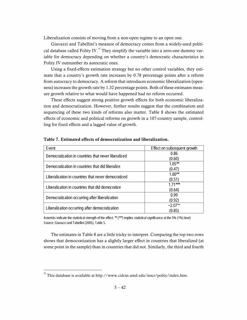
5 – 42

Liberalization consists of moving from a non-open regime to an open one. Giavazzi and Tabellini’s measure of democracy comes from a widely-used politi-

cal database called Polity IV.35

They simplify the variable into a zero-one dummy var-iable for democracy depending on whether a country’s democratic characteristics in Polity IV outnumber its autocratic ones. Using a fixed-effects estimation strategy but no other control variables, they esti-mate that a country’s growth rate increases by 0.78 percentage points after a reform from autocracy to democracy. A reform that introduces economic liberalization (open-ness) increases the growth rate by 1.32 percentage points. Both of these estimates meas-ure growth relative to what would have happened had no reform occurred. These effects suggest strong positive growth effects for both economic liberaliza-tion and democratization. However, further results suggest that the combination and sequencing of these two kinds of reforms also matter. Table 8 shows the estimated effects of economic and political reforms on growth in a 107-country sample, control-ling for fixed effects and a lagged value of growth.

Table 7. Estimated effects of democratization and liberalization.

Event Effect on subsequent growth

Democratization in countries that never liberalized 0.86 (0.60)

Democratization in countries that did liberalize 1.05** (0.47)

Liberalization in countries that never democratized 1.00** (0.51)

Liberalization in countries that did democratize 1.71*** (0.64)

Democratization occurring after liberalization 0.99 (0.92)

Liberalization occurring after democratization −2.07** (0.85)

Asterisks indicate the statistical strength of the effect. ** (***) implies statistical significance at the 5% (1%) level. Source: Giavazzi and Tabellini (2005), Table 5. The estimates in Table 8 are a little tricky to interpret. Comparing the top two rows shows that democratization has a slightly larger effect in countries that liberalized (at some point in the sample) than in countries that did not. Similarly, the third and fourth

35

This database is available at http://www.cidcm.umd.edu/inscr/polity/index.htm.

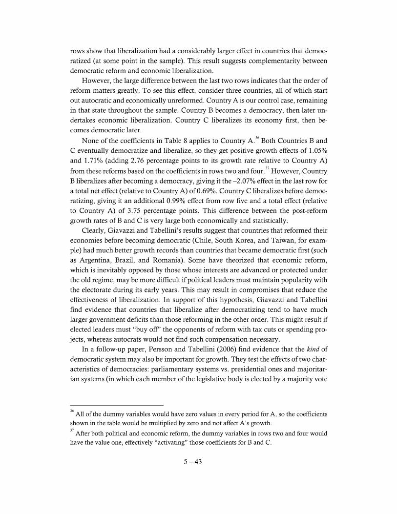
5 – 43

rows show that liberalization had a considerably larger effect in countries that democ-ratized (at some point in the sample). This result suggests complementarity between democratic reform and economic liberalization. However, the large difference between the last two rows indicates that the order of reform matters greatly. To see this effect, consider three countries, all of which start out autocratic and economically unreformed. Country A is our control case, remaining in that state throughout the sample. Country B becomes a democracy, then later un-dertakes economic liberalization. Country C liberalizes its economy first, then be-comes democratic later.

None of the coefficients in Table 8 applies to Country A.36

Both Countries B and C eventually democratize and liberalize, so they get positive growth effects of 1.05% and 1.71% (adding 2.76 percentage points to its growth rate relative to Country A)

from these reforms based on the coefficients in rows two and four.37

However, Country B liberalizes after becoming a democracy, giving it the –2.07% effect in the last row for a total net effect (relative to Country A) of 0.69%. Country C liberalizes before democ-ratizing, giving it an additional 0.99% effect from row five and a total effect (relative to Country A) of 3.75 percentage points. This difference between the post-reform growth rates of B and C is very large both economically and statistically. Clearly, Giavazzi and Tabellini’s results suggest that countries that reformed their economies before becoming democratic (Chile, South Korea, and Taiwan, for exam-ple) had much better growth records than countries that became democratic first (such as Argentina, Brazil, and Romania). Some have theorized that economic reform, which is inevitably opposed by those whose interests are advanced or protected under the old regime, may be more difficult if political leaders must maintain popularity with the electorate during its early years. This may result in compromises that reduce the effectiveness of liberalization. In support of this hypothesis, Giavazzi and Tabellini find evidence that countries that liberalize after democratizing tend to have much larger government deficits than those reforming in the other order. This might result if elected leaders must “buy off” the opponents of reform with tax cuts or spending pro-jects, whereas autocrats would not find such compensation necessary. In a follow-up paper, Persson and Tabellini (2006) find evidence that the kind of democratic system may also be important for growth. They test the effects of two char-acteristics of democracies: parliamentary systems vs. presidential ones and majoritar-ian systems (in which each member of the legislative body is elected by a majority vote

36

All of the dummy variables would have zero values in every period for A, so the coefficients shown in the table would be multiplied by zero and not affect A’s growth. 37

After both political and economic reform, the dummy variables in rows two and four would have the value one, effectively “activating” those coefficients for B and C.

5 – 44

in a district) vs. proportional-representation systems (in which parties are allocated seats in proportion to their national or regional vote total). Persson and Tabellini find no significant difference in growth outcomes between majoritarian and proportional systems, but they do estimate that the growth rate is 1.61 percentage points lower in parliamentary democracies than in presidential ones. Other results suggest that parliamentary systems are more likely to pursue economic liberalization than presidential ones (though these reforms, occurring after democrati-zation, have small effects) and are more likely to increase government consumption (the buying-off-opponents effect). Persson and Tabellini argue that this “binge spend-ing” associated with economic reform accompanied by a surge in government con-sumption spending may cause distortions that lower economic growth. In another recent paper, Besley, Persson, and Sturm (2006) examine the effects of political competition on growth, using evidence from the U.S. states. They develop a theoretical model to show that greater competitiveness of political races might lead parties to nominate better candidates, who then enact better policies once elected. They use the passage of the Voting Rights Act, which initiated the destruction of traditional Democratic dominance in the South, as a natural experiment to measure the effect of increased competition between parties on economic policies and growth. They find that greater political competition seems to lead to better governors, better economic policies, and higher state income growth. While many authors have included political institutions such as democracy and rule of law in growth regressions, the causality is ambiguous. Do countries with “good” political institutions grow faster or do fast-growing countries develop better institutions, or both? In order to attempt to determine causality, we need to find a variable that affects institutions but that does not separately affect growth. Such a var-iable could be used as an instrumental variable in estimation. Acemoglu, Johnson, and Robinson (2001) show that European colonies located in parts of the world where the colonists had low mortality rates developed better institutions than other colonies. Where colonist mortality was low, they tended to settle in the countries and establish European-like institutions; where mortality rates were high, they did not settle and merely extracted resources from the colony and colonists. Because colonist mortality rates affect institutions but can be assumed to have no direct effect on current income and growth, they are suitable instrumental variables for use in disentangling the cau-sality between institutions and growth. Using these methods, Acemoglu, Johnson, and Robinson find strong causality running from political institutions to growth.

Inequality and growth Another question that has been of great interest to economists and policymakers is the relationship between economic growth and income inequality within countries. Causal effects in either direction are possible: having more inequality may be good or

5 – 45

bad for a country’s growth prospects and, conversely, growing faster may increase or decrease inequality. Persson and Tabellini (1994) provide evidence on the effects of inequality on growth. The theoretical growth models we have studied are all representative-agent models in which everyone is the same, so these models cannot tell us anything about possible effects of inequality. Persson and Tabellini build an overlapping-generations model in which newborn agents vary in their endowment of skills that can be sold in the labor market. Agents not only interact in the usual way in economic markets, but they also decide on a policy parameter analogous to a redistributive tax rate through democratic political interaction. As is common in such models, it is the preferences of

the median voter that determine the political outcome.38

The distribution of skills is assumed to have a long but thin tail at the top end (a few extremely high-skilled people) and a short but thick tail at the bottom (many peo-ple with skills below the mean, but not too far below). This implies that the median of the distribution lies below the mean, the latter being dragged upward by the dispropor-tionate effect of averaging in the few extremely highly skilled people. A reduction in endowment inequality would push the median endowment upward toward the mean, which would reduce the preference of the median voter for tax-based redistribution of income. Since high redistributive taxes discourage investment, they lower the equilibrium growth path. A reduction in (before-tax) income inequality thus lowers the public’s (median voter’s) demand for high taxes and raises the steady-state growth path. Persson and Tabellini use two data samples to test the hypothesis that inequality lowers growth. The first is a historical sample of data since 1830 on nine now-devel-oped countries: Austria, Denmark, Finland, Germany, Norway, Sweden, the United States, and the United Kingdom. Each country is observed (if data are available) over 20-year periods beginning with 1830–1850 and ending with 1970–1985. (The last pe-riod spans only 15 years because data through 1990 were not available at the time the paper was written.) They measure income inequality as the share of income earned by households in the top 20 percent of the income distribution. They expect an increase in this variable to reduce growth. However, not all those earning income have been allowed to vote through much of the sample period. To the extent that it is poorer voters who are disenfranchised, the median voter (as distinct from the median earner) has a higher income, which will lead to a lower level of redistributive taxes and higher growth. Thus, they expect a positive growth effect from their variable measuring the share of the population that is

38

The median voter is the one who has an endowment higher than 50% of the population and lower than 50%.

5 – 46

disenfranchised. To control for convergence and human-capital effects, they also in-clude a schooling variable and a variable measuring the gap between the country’s level of per-capita income at the beginning of the 20-year period and the highest in-come level in the world at that time. Persson and Tabellini’s results support their hypothesis that greater inequality leads to lower growth. An increase of 0.07 in the share of income earned by the top 20 percent of the population (which is an increase of one standard deviation in this vari-able) lowers growth by about one-half percentage point. They find a slightly negative but statistically insignificant effect of disenfranchisement. They attribute this unex-pected result to the lack of variation in this variable in their sample. Persson and Tabellini second sample uses a larger group of countries over the post-war period. For this sample, they measure income equality/inequality by the share of income earned by the middle quintile (40th to 60th percentiles of income-earners). An increase in this share corresponds to an increase in equality of incomes, so they expect it to have a positive effect on growth. Again, their results support the hypothesis that increases in income equality lead to increases in growth. As in the other sample, a one-standard-deviation increase in the equality variable leads to a growth rate that is higher by about one-half percentage point. The evidence of Persson and Tabellini suggests that inequality is bad for growth, but what about the effect of growth on inequality? Do the income distributions in growing countries tend to get more equal or more unequal? Dollar and Kraay (2002) look at the effects of growth on the incomes of the poorest members of society. Specifically, Dollar and Kraay examine the effect of growth and growth-enhancing policies on the incomes of the lowest 20 percent of the population. Using panel data by decades on growth in 92 countries, they find no effect of either growth or the com-mon economic liberalization policies used to stimulate growth on the share of income earned by the bottom quintile. This means that while growth has not helped to lift the poorest members of society in relative terms, it has raised their incomes in the same proportion that it has raised those of wealthier people. Thus, Dollar and Kraay find evidence in support of what is sometimes called the “high-tide-lifts-all-boats” hypoth-esis.

Studies of cross-country income differences To test for level effects of human capital and other variables we can examine the association between levels of human capital and levels of per capita real income. Romer reviews two major studies of cross-country differences in income or productivity in section 4.2. In this section, we consider some additional details from these two studies. Both the paper by Hall and Jones (1999) and the study by Klenow and Rodriguez-Clare (1997) adopt a growth-accounting approach rather than the econometric method of Barro and Lee. To estimate stocks of human capital, both studies rely on the Barro-

5 – 47

Lee estimates of educational attainment. However, to employ these numbers in a growth-accounting framework the raw averages for primary, secondary, and higher education per person must be reduced to a single human-capital number for each coun-try. How can we combine or aggregate the amount (value) of human capital embodied in people with a high school degree together with people with no high school or other education levels? The answer is that we should aggregate workers together based on their relative productivity levels. If workers with a high school degree are twice as pro-ductive as workers with no high school, then they should count for twice as much human capital. How, then, might we estimate the relative productivity levels of people with dif-ferent education level? The method chosen by both studies is to take advantage of many years of empirical research in labor economics where economists have at-tempted to estimate the effect of education on wages. In a competitive market with perfect information, each worker should be paid a wage equal to his or her marginal productivity. If relative wages accurately reflect the marginal productivity of various kinds of labor, then the wage distribution across education levels should mirror the productivity distribution. Hall and Jones use the results of studies of the wage distri-bution for many countries to aggregate workers of various education levels into a single human-capital aggregate for each country. Klenow and Rodriguez-Clare go a step far-ther by attempting to correct for quality differences between the schooling received in different countries. The main result of both studies emphasizes that differences in human capital are an important part of international income differences, but that a large residual remains unexplained. In other words, human and physical capital differences can explain only part of the differences between rich and poor countries. A larger share is due to produc-tivity differences that are not explained within the traditional growth-accounting framework—analogous to the Solow residual discussed in our Chapter 2.

Rent seeking and growth One key determinant of technological progress is how many students study aca-demic fields that contribute to it: so-called STEM (science, technology, engineering, mathematics) fields. While students’ aptitudes and interests undoubtedly play a central (and perhaps dominant) role in deciding fields of study, many students are influenced by the prospective incomes they might earn in various fields. If the economic system provides high rewards for scientists, we expect more stu-dents to study science. If incomes are higher for financial professionals or lawyers, more students would be tempted in those directions. An earlier version of the Romer textbook included a model of “production, predation, and protection.” In this model, individuals chose whether to produce output or to “steal” someone else’s production.

5 – 48

This theft need not be illegal; it may be rent-seeking or lobbying activity that seeks legal forms of redistribution such as subsidies or tax benefits. It could also be bribery in order to influence legal or legislative decisions. The key is that this non-production activity does not generate any benefit for society as a whole, it just redistributes benefit to the “predator.” The model shows that in the presence of rent seekers, those who choose to be pro-ducers may find it useful to engage in “protection” activities that attempt to minimize the usurpation of their output by rent seekers. This could take the form of counter-lobbying or (in the case of actual theft) of taking costly security measures. The decision whether to be a producer or a predator is based on the expected re-turns to each activity. The more predators are around, the less any individual predator will earn (because there are fewer producers) and the more each producer will resort to protection. Equilibrium output in the economy depends on how many people choose to produce and how much of their activity is devoted to protection rather than actual production. This has clear relation to the “institutions” argument about growth. In some econ-omies, the institutional setup makes predation very difficult because laws are enforced, corruption is rare, and penalties are severe. In other places, predation is relatively easy, safe, and lucrative. Kevin Murphy, Andrei Shleifer, and Robert Vishny attempted to look at the

growth effects of rent seeking.39

They used the share of college students enrolled in law schools and the share enrolled in engineering schools to measure the relative attrac-tiveness of rent seeking vs. production. Table 9 shows the results of a regression that follows a standard model for cross-country growth regressions, but with law and engi-neering enrollments added. The dependent variable is the per capita GDP growth rate over 1970 to 1985. Their sample includes the 55 countries that had at least 10,000 college students in 1970. The initial GDP variable and the measures of investment, primary school enroll-ment, government consumption, and revolutions have the expected effects, though not

all are statistically significant.40

The coefficients on the shares of engineering and law students support the hypoth-esis that rent-seeking activities reduce growth, although the statistical significance of the coefficients is marginal at best. The authors argue that the effect is actually stronger than the magnitude of the coefficients shown in Table 9 because countries with more engineering and fewer law students also have higher levels of investment. Adding in

39

Murphy, Shleifer, and Vishny (1991). 40

Note that this study uses primary school enrollment rather than the Barro-Lee school attain-ment measures. The Barro-Lee measures had not yet been published at the time the Murphy, Shleifer, and Vishny study was done.

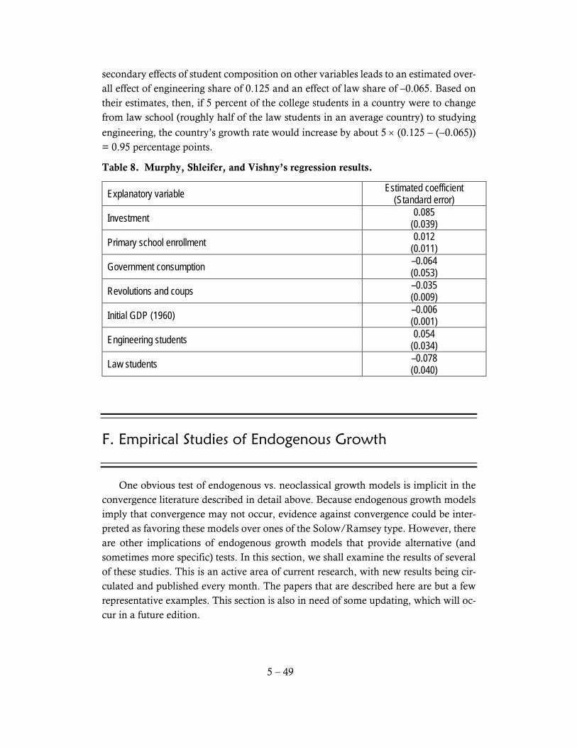
5 – 49

secondary effects of student composition on other variables leads to an estimated over-all effect of engineering share of 0.125 and an effect of law share of –0.065. Based on their estimates, then, if 5 percent of the college students in a country were to change from law school (roughly half of the law students in an average country) to studying

engineering, the country’s growth rate would increase by about 5 × (0.125 − (−0.065)) = 0.95 percentage points.

Table 8. Murphy, Shleifer, and Vishny’s regression results.

Explanatory variable Estimated coefficient (Standard error)

Investment 0.085 (0.039)

Primary school enrollment 0.012 (0.011)

Government consumption –0.064 (0.053)

Revolutions and coups –0.035 (0.009)

Initial GDP (1960) –0.006 (0.001)

Engineering students 0.054 (0.034)

Law students –0.078 (0.040)

F. Empirical Studies of Endogenous Growth

One obvious test of endogenous vs. neoclassical growth models is implicit in the convergence literature described in detail above. Because endogenous growth models imply that convergence may not occur, evidence against convergence could be inter-preted as favoring these models over ones of the Solow/Ramsey type. However, there are other implications of endogenous growth models that provide alternative (and sometimes more specific) tests. In this section, we shall examine the results of several of these studies. This is an active area of current research, with new results being cir-culated and published every month. The papers that are described here are but a few representative examples. This section is also in need of some updating, which will oc-cur in a future edition.

5 – 50

Evidence on growth vs. level effects of economic changes Endogenous growth implies that changes in such parameters as the saving rate, the share of resources allocated to R&D, and government policies that affect these parameters should have effects not only on the level of per-capita income (as in the Solow model) but on the rate of growth. For example, in Paul Romer’s R&D model (see equation (3.34) on page 126 of D. Romer’s text), the rate of growth of technology depends on aL, which is the share of labor devoted to the R&D sector. Jones (1995) argues that under endogenous growth, any permanent change in a variable such as government fiscal policy should lead to a permanent change in the trend growth rate. He finds that there have been significant changes in fiscal policy variables, but no corresponding changes in growth, so he rejects endogenous growth. Jones’s study was criticized by subsequent authors for relying too much on the indi-vidual behavior of the growth and investment variables and not adequately investigat-ing the time-series relationship between them. Paul Evans (1997) examined government consumption in detail for 92 countries. His results are strikingly consistent: growth effects (endogenous growth) are supported in only three of the 92 countries. Evans concludes that the evidence supports the kind of exogenous growth found in the Solow model rather than the self-reinforcing endog-enous growth implied by the modern models with constant returns to produced inputs. However, using long-sample data for the United States and United Kingdom, Kocherlakota and Yi (1997) are able to reject the hypothesis that growth is exogenous using different government spending variables. Where Evans used government con-sumption, they use a disaggregated set of government variables. They find permanent effects for both public (government-provided) capital and tax-rate variables. This rein-forces their earlier result from Kocherlakota and Yi (1996), for which they found that

government investment had permanent effects in the United States.41

Evidence on the effects of private human capital vs. public knowledge Peter Klenow (1998) performed an empirical test to discriminate between the two kinds of models discussed in Romer’s Chapter 3 and 4. Recall that in the R&D models of the first part of the chapter, knowledge is a public good that increases the produc-tivity of every producer in every industry once it has been created. In contrast, the hu-man-capital model implies that the enhanced productivity from human capital is em-bodied in workers. Only producers and industries that employ labor having the human capital will see increased productivity. Klenow noted that in the human-capital model, productivity growth should be higher in labor-intensive industries than in industries that employ less labor, since they will benefit more from human capital investment.

41

See Poot (2000) for a useful survey of the literature on government effects on growth.

5 – 51

However, if knowledge is general (as in the R&D model) then all industries should benefit equally. Klenow uses data for 450 detailed manufacturing industries from the NBER Man-ufacturing Productivity Database to examine the connection between productivity growth and labor intensity. He finds that industries with high labor intensity, however measured, tend to have lower rather than higher productivity growth, which is evidence for the general knowledge model over the specific human-capital model. In fact, it supports a model in which knowledge is embodied in capital rather than in labor. He expresses the essence of his result with the following very accessible anecdote in his conclusion:

Using the human capital I gleaned from a high school typing class, I could have typed this paper on the 1982-vintage typewriter I received for my high school graduation. Correcting spelling errors would have been a slow and tedious process. In contrast, the word processor I used allowed me to correct spelling errors with only a few commands. My knowledge of the required keystrokes surely represents human capital. But I did not need to understand the software or hardware that re-sponded to my keystrokes. With little change in my typing human cap-ital, the ideas embedded in my computer dramatically raised my productivity in correcting typos.

Industry evidence in the NBER Database suggests that this anecdote may be more the rule than the exception. Industries with rapid produc-tivity growth are not intensive in overall labor, nonproduction labor, or high wage labor. I could not explain these facts with either a general or industry-specific human capital model. … In the data rapid [total factor productivity] growth industries have rapidly declining … capital and materials prices, favoring [a theory based on] industry-specific ideas embodied in capital and intermediate inputs. [Klenow (1998)]

However, Klenow is careful to point out that theories based on rival human capital and those relying on nonrival knowledge could be complements rather than substitutes in explaining productivity growth. Although his evidence fails to find strong evidence of human-capital-based growth in U.S. manufacturing, that does not mean that it might not be of great importance in non-manufacturing industries or in other coun-tries.

5 – 52

G. Suggestions for Further Reading

Overviews of growth and empirical results Barro, Robert, and Xavier Sala-i-Martin, Economic Growth, 2nd ed., (Cambridge, Mass.:

MIT Press, 2004). (Chapters 10 through 12 have extensive empirical content.) Durlauf, Steven N., and Danny T. Quah, “The New Empirics of Economic Growth,”

in Handbook of Macroeconomics, Volume 1A, edited by J. B. Taylor and M. Wood-ford (Amsterdam: Elsevier Science, 1999).

Various authors, Handbook of Economic Growth, Volume 1A, (Amsterdam: North-Hol-land, 2005), Chapters 8 – 11.

Selected growth accounting studies Barro, Robert, and Xavier Sala-i-Martin, Economic Growth, 2nd ed., (Cambridge, Mass.:

MIT Press, 2004), Chapter 10. (A survey of growth accounting results.) Denison, Edward, Accounting for United States Economic Growth, 1929–1969 (Washing-

ton, D.C.: Brookings Institution, 1967). (An old but very detailed growth account-ing study, which provides lots of detail on the methodology.)

Denison, Edward, Trends in American Economic Growth, 1929–1982 Washington, D.C.: Brookings Institution, 1985). (A more up-to-date analysis using the same method-ology.)

Jorgenson, Dale W., Frank M. Gollup, and Barbara M. Fraumeni, Productivity and U.S. Economic Growth (Cambridge, Mass.: Harvard University Press, 1987). (A very detailed study of total-factor-productivity growth in various industries.)

Maddison, Angus, Dynamic Forces in Capitalist Development (Oxford: Oxford University Press, 1991). (Long-term growth accounting for a set of now-industrialized econ-omies.)

Maddison, Angus, The World Economy: A Millennial Perspective, (Paris: OECD, 2001). (An attempt to measure growth over 10 centuries.)

H. Studies Referenced in Text

Acemoglu, Daron, Simon Johnson, and James Robinson. 2001. The Colonial Origins of Comparative Development: An Empirical Investigation. American Economic Review 91 (5):1369-1401.

5 – 53

Barro, Robert J., and Jong Wha Lee. 1993. International Comparisons of Educational Attainment. Journal of Monetary Economics 32 (3):363-94.

———. 1994. Sources of Economic Growth. Carnegie Rochester Conference Series on Public Policy 40:1-46.

———. 2000. International Data on Educational Attainment: Updates and Implications. Cambridge, Mass.: National Bureau of Economic Research.

Barro, Robert J., and Xavier Sala-i-Martin. 1991. Convergence across States and Regions. Brookings Papers on Economic Activity (1):107-58.

———. 1992. Convergence. Journal of Political Economy 100 (2):223-51. ———. 1995. Economic Growth. New York: McGraw-Hill. ———. 2004. Economic Growth. 2nd ed. Cambridge, Mass.: MIT Press. Basu, Susanto, and David N. Weil. 1998. Appropriate Technology and Growth.

Quarterly Journal of Economics 113 (4):1025-54. Baumol, William J. 1986. Productivity Growth, Convergence, and Welfare: What

the Long-run Data Show. American Economic Review 76 (5):1072-85. Besley, Timothy, Torsten Persson, and Daniel Sturm. 2006. Political Competition

and Economic Performance: Theory and Evidence from the United States. Paper read at American Economic Association Annual Meetings, January, at Boston, Mass.

Bianchi, Marco. 1997. Testing for Convergence: Evidence from Non-parametric Multimodality Tests. Journal of Applied Econometrics 12 (4):393-409.

Cohen, Daniel, and Marcelo Soto. 2007. Growth and Human Capital: Good Data, Good Results. Journal of Economic Growth 12 (1):51-76.

De Long, J. Bradford. 1988. Productivity Growth, Convergence, and Welfare: Comment. American Economic Review 78 (5):1138-54.

Denison, Edward F. 1985. Trends in American Economic Growth, 1929-1982. Washington, D.C.: Brookings Institution.

Dollar, David, and Aart Kraay. 2002. Growth is Good for the Poor. Journal of Economic Growth 7 (3):195-225.

Durlauf, Steven N., and Danny T. Quah. 1999. The New Empirics of Economic Growth. In Handbook of Macroeconomics, edited by J. B. Taylor and M. Woodford. Amsterdam: Elsevier Science.

Evans, Paul. 1997. Government Consumption and Growth. Economic Inquiry 35 (2):209-217.

Feenstra, Robert C., Robert Inklaar, and Marcel P. Timmer. 2015. The Next Generation of the Penn World Table. American Economic Review 105 (10):3150-82.

Friedman, Thomas L. 2005. The World Is Flat: A Brief History of the Twenty-First Century. New York: Farrar, Straus, and Giroux.

Giavazzi, Francesco, and Guido Tabellini. 2005. Economic and Political Liberalization. Journal of Monetary Economics 52 (7):1297-1330.

Graham, Bryan S., and Jonathan R. W. Temple. 2006. Rich Nations, Poor Nations: How Much Can Multiple Equilibria Explain? Journal of Economic Growth 11 (1):5-41.

Hall, Robert E., and Charles I. Jones. 1999. Why Do Some Countries Produce So Much More Output Per Worker Than Others? Quarterly Journal of Economics 114 (1):83-116.

5 – 54

Higgins, Matthew J., Daniel Levy, and Andrew T. Young. 2006. Growth and Convergence across the United States: Evidence from County-Level Data. Review of Economics and Statistics 88 (4):671-681.

Jones, Charles I. 1995. Time Series Tests of Endogenous Growth Models. Quarterly Journal of Economics 110 (2):495-525.

Jorgenson, Dale W. 2001. Information Technology and the U.S. Economy. American Economic Review 91 (1):1-32.

Jorgenson, Dale W., and Khuong M. Vu. 2016. The ICT Revolution, World Economic Growth, and Policy Issues. Telecommunications Policy 40:383-397.

Klenow, Peter J. 1998. Ideas versus Rival Human Capital: Industry Evidence on Growth Models. Journal of Monetary Economics 42 (1):3-23.

Klenow, Peter J., and Andres Rodriguez-Clare. 1997. The Neoclassical Revival in Growth Economics: Has It Gone Too Far? In NBER Macroeconomics Annual 1997, edited by B. S. Bernanke and J. J. Rotemberg. Cambridge and London: MIT Press.

Kocherlakota, Narayana R., and Kei Mu Yi. 1996. A Simple Time Series Test of Endogenous vs. Exogenous Growth Models: An Application to the United States. Review of Economics and Statistics 78 (1):126-134.

———. 1997. Is There Endogenous Long-Run Growth? Evidence from the United States and the United Kingdom. Journal of Money, Credit and Banking 29 (2):235-62.

Kraay, Aart, and Claudio Raddatz. 2007. Poverty Traps, Aid, and Growth. Journal of Development Economics 82 (2):315-347.

Kurtz, Marcus J., and Andrew Schrank. 2007. Growth and Governance: Models, Measures, and Mechanisms. Journal of Politics 69 (2):538-554.

Maddison, Angus. 1991. Dynamic Forces in Capitalist Development: A Long-Run Comparative View. Oxford: Oxford University Press.

———. 2001. The World Economy: A Millennial Perspective. Paris: OECD. Mankiw, N. Gregory, David Romer, and David N. Weil. 1992. A Contribution to

the Empirics of Economic Growth. Quarterly Journal of Economics 107 (2):407-37.

Measuring Economies: The Trouble with GDP. 2016. Economist, April 30, 2016. Mokyr, Joel. 1990. The Lever of Riches: Technological Creativity and Economic Progress.

Oxford and New York: Oxford University Press. Murphy, Kevin M., Andrei Shleifer, and Robert W. Vishny. 1991. The Allocation of

Talent: Implications for Growth. Quarterly Journal of Economics 106 (2):503-30.

Persson, Torsten, and Guido Tabellini. 1994. Is Inequality Harmful for Growth? American Economic Review 84 (3):600-621.

———. 2006. Democracy and Development: The Devil in the Details. Cambridge, Mass.: National Bureau of Economic Research.

Poot, Jacques. 2000. A Synthesis of Empirical Research on the Impact of Government on Long-Run Growth. Growth and Change 31 (4):516-546.

Pritchett, Lant. 1997. Divergence, Big Time. Journal of Economic Perspectives 11 (3):3-17.

Przeworski, Adam, and Fernando Limongi. 1993. Political Regimes and Economic Growth. Journal of Economic Perspectives 7 (3):51-60.

5 – 55

Quah, Danny. 1993. Empirical Cross-Section Dynamics in Economic Growth. European Economic Review 37 (2-3):426-34.

Rosenberg, Nathan. 1982. Inside the Black Box: Technology and Economics. Cambridge: Cambridge University Press.

Sachs, Jeffrey D., John W. McArthur, Guido Schmidt-Traub, Margaret Kruk, Chandrika Bahadur, Michael Faye, and Gordon McCord. 2004. Ending Africa's Poverty Trap. Brookings Papers on Economic Activity 2004 (1):117-216.

Sachs, Jeffrey D., and Andrew M. Warner. 1995. Economic Reform and the Process of Global Integration. Brookings Papers on Economic Activity (1):1-95.

Sala-i-Martin, Xavier. 1997. I Just Ran Two Million Regressions. American Economic Review 87 (2):178-83.