a program for kriging water level data using hydrologic ...a program for kriging water level data...
TRANSCRIPT

A Program for Kriging Water Level Data using
Hydrologic Drift Terms
User manual
Version 3.0 - Beta

DESCRIPTION OF THE KT3D_H2O PROGRAM SUITE
INTRODUCTION......................................................................................................................... 1
ABOUT THIS DOCUMENT.............................................................................................................. 2
UNDERLYING CODES .................................................................................................................... 2
SUPPORTED INPUTS AND OUTPUTS .............................................................................................. 2
DISCLAIMER................................................................................................................................. 3
TECHNICAL SUPPORT................................................................................................................... 3
INSTALLING AND STARTING KT3D_H2O.......................................................................... 4
CREATING A NEW PROJECT................................................................................................. 6
KRIGING TO GENERATE A GRID......................................................................................... 7
PREPARING DATA......................................................................................................................... 7
IMPORTING DATA ......................................................................................................................... 8
SETTING GRID PARAMETERS......................................................................................................... 9
SETTING KRIGING PARAMETERS ................................................................................................ 10
SELECTING KRIGING TYPES AND DRIFTS..................................................................................... 11
2D Well function drift ........................................................................................................... 11
2D Horizontal line sink/source drift ..................................................................................... 12
2D Circular pond.................................................................................................................. 13
SETTING VARIOGRAM PARAMETERS........................................................................................... 14
RUNNING THE KRIGING.............................................................................................................. 16
SINGLE EVENT KRIGING ............................................................................................................. 16
MULTI EVENT KRIGING.............................................................................................................. 17
EXPORTING KRIGING RESULTS ................................................................................................... 18
IMPORTING KRIGING RESULTS .................................................................................................... 18

APPEND NEW EVENTS ................................................................................................................ 20
PARTICLE TRACKING........................................................................................................... 21
SETTING PARTICLE TRACKING PARAMETERS .............................................................................. 21
SETTING PARTICLE STARTING LOCATIONS.................................................................................. 22
Running particle tracking ..................................................................................................... 25
HYDRAULIC CAPTURE ZONE ANALYSIS........................................................................ 27
EXPORTING HYDRAULIC CAPTURE ZONE ANALYSIS RESULTS.................................................... 28
REFERENCES............................................................................................................................ 29
APPENDIX A KT3D_H2O INPUT FORMATS..................................................................... 30
APPENDIX B BINARY FILE FORMATS ............................................................................. 33
APPENDIX C ARCINFO ASCII GRID FILES FORMATS ................................................. 35
Attachment 1:
KT3D_H2O v3.0 A Program for Kriging Water Level Data using Hydrologic Drift Terms:
Theoretical Documentation
Attachment 2:
Documentation and Verification Package for TransientTracker

1
Introduction
KT3D_H2O Version 3.0 is a graphical user interface (GUI) that combines various
programs to generate gridded maps of water level elevations, particle tracks and capture
zones. These tools combine geosatistical and hydrological sciences to allow the user to
generate map-based hydrogeologic analyses outputs without having to revert to numerical
or analytical models.
KT3D_H2O is developed as a plug-in application under the open-source GIS foundation
MapWindow. It allows the user to generate gridded maps of water level elevations that
include the following elements that have important influence on the shape of the mapped
surface and are usually ignored by other gridding software applications:
• Point Sink or Source of Known Strength: accounts for mounding (or drawdown) in response to injection (or extraction) at a known rate at one or more wells.
• Horizontal Line Sink or Source of Known Strength: account for mounding (or drawdown) in response to horizontal linear features of known extraction (injection) rate, such as interception trenches or infiltration galleries; and
• Circular Leaking Pond of Known Strength: accounts for the potentiometric response of a water table (unconfined) aquifer to infiltration through the base of a circular pond.
The available drift terms can be applied simultaneously, i.e. a single gridded surface may
contain point sinks or sources, horizontal line sink or circular leaking pond. In addition,
in order to account for heterogeneity, different groupings of the drift elements are
possible so that scaling provided by universal kriging is performed independently on each
group to obtain a best fit (e.g. wells located in a high transmissivity zone can be assigned
to Point Sink Drift Term 1 and wells located in a low transmissivity zone are placed in
Point Sink Drift Term 2).
These gridded surfaces can be used to complete the following types of hydrogeologic
analyses maps for single or multiple events:
• maps of water level elevations; • maps showing particle traces (particle tracking); and • maps of particle capture (capture zone analysis including capture frequency
maps)

2
About this Document
This document describes the various functions of the KT3D_H2O graphical user
interface. Attachments 1 and 2 provide the theoretical documentation for the underlying
codes: KT3D_H2O and Transient Tracker. This document constitutes a Beta version
release that is not complete or fully tested.
Underlying codes
KT3D_H2O Version 3.0 is written in VB.Net and combines the latest version of linear-
log kriging program KT3Ddll.dll and Transient Tracker. First version for kriging with
linear-log drift, called KT3D_L1, is developed by modifying popular GSLIB KT3D
kriging code then fortran program is compiled as a Dynamic Link Library (DLL), which
is executed using a Visual Basic UI called “kt3d_loglin”.
The MapWindow application is a free and extensible geographic information system
(GIS) that can be used to distribute data to others, and to develop and distribute custom
spatial data analyses. MapWindow includes standard GIS data visualization features as
well as DBF attribute table editing, shapefile editing, and grid importing and conversion.
MapWinGIS ActiveX includes a GIS API for shapefile and grid data with many built in
GIS functions.
Supported Inputs and Outputs
The KT3D_H2O GUI supports importing data from Microsoft Excel versions 2000-2007
(*.xls, *.xlsx, *. xlsb and *.xlsm) files, Microsoft Access versions 2000-2007 (*.mdb and
*.accdb) files, ESRI Shape Files (*.shp) and ASCII. It offers several post-processing
options for the calculated grids:
Selected Output Format Grid Format Particle Line Format (1,2) SurferTM ASCII SurferTM v7 Grid
ESRI / ArcMAPTM ASC ESRI Shape (SHP) file 1. Times associated with pathlines are written in units that correspond with the specified
hydraulic conductivity units in the GUI’s {Part.Track} tab. 2. All methods result in the production of the file “CAPTURE.OUT” 3. Appendix C describes the ASC grid format

3
Disclaimer
This software and documentation is provided "AS IS", without warranty of any kind,
including without limitation the warranties of merchantability, fitness for a particular
purpose and non-infringement. The entire risk and responsibility as to the quality and
performance of the Software is borne by the user. The author(s) disclaim all other
warranties.
The following text from the GSLIB KT3D program details the copyright and distribution
rights pertaining to the GSLIB programs.
“Copyright (C) 1996, The Board of Trustees of the Leland Stanford Junior
University. All rights reserved.
The programs in GSLIB are distributed in the hope that they will be useful, but
WITHOUT ANY WARRANTY. No author or distributor accepts responsibility to
anyone for the consequences of using them or for whether they serve any particular
purpose or work at all, unless he says so in writing. Everyone is granted permission
to copy, modify and redistribute the programs in GSLIB, but only under the condition
that this notice and the above copyright notice remain intact.”
The current release constitutes a Beta version that has not been fully tested.
Technical Support
Technical support regarding use of the graphical user interface can be obtained by writing

4
Installing and starting KT3D_H2O
Installation Requirements:
• It is assumed that KT3D_H2O users already have some basic understanding of
kriging techniques and GIS concepts.
• It is assumed that user already has installed the latest version of MapWindow,
which can be downloaded at:
(http://www.mapwindow.org/download.php?show_details=1)
• The latest version of the MapWindow book can be purchased or downloaded free
from http://www.lulu.com/ Also, the 1st edition of book is included in KT3D
installation file
To install KT3D_H2O using the setup file, follow these three steps:
1. Download the installation program: KT3D_H20_Setup.exe from: www.sspa.com
2. Run the installation program, following instructions on the screen. The destination
folder must be the MapWindow root folder, usually “C:\ProgramFiles\MapWindow”.
3. The setup program installs all necessary Dynamic Link Library files (dll’s), user’s
manuals and sample files into appropriate MapWindow folders.

5
After installing KT3D_H20, open MapWindow. Click on “Plug-Ins” from the
MapWindow toolbar, and select “KT3D_H20”. This will
add KT3D_H2O to the MapWindow toolbar. If
“KT3D_H2O” is not listed under “Plug-Ins”, make sure
that the file “SSPA Tools.dll” exists in MapWindow
plugins folder usually,
“C:\ProgramFiles\MapWindow\Plugins\” or
“C:\ProgramFiles\MapWindow\Plugins\KT3D_H2O”.
The KT3D_H2O button should now appear on your
MapWindow Menu bar. Click on this button to open the
KT3D_H20 User Interface (UI):
6
Creating a new project
In order to use KT3D_H2O, you first need to create a new project or open an existing
one. There are two types of projects that can be used for the kriging: the Single Event
type for the kriging one data set, and Multi Event type for kriging multiple data sets.
The Single event type is used to create a single result; for example, a single map of
overall average water elevation. The Multi Event type is used to create multiple results
corresponding to multiple events; for example, this type would be used to create several
maps, each showing water levels from a different sampling event.
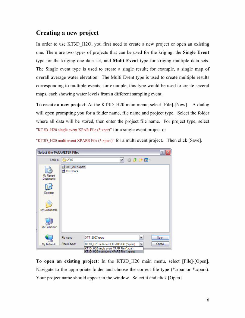
To create a new project: At the KT3D_H20 main menu, select [File]-[New]. A dialog
will open prompting you for a folder name, file name and project type. Select the folder
where all data will be stored, then enter the project file name. For project type, select
”KT3D_H20 single event XPAR File (*.xpar)” for a single event project or
"KT3D_H20 multi event XPARS File (*.xpars)” for a multi event project. Then click [Save].
To open an existing project: In the KT3D_H20 main menu, select [File]-[Open].
Navigate to the appropriate folder and choose the correct file type (*.xpar or *.xpars).
Your project name should appear in the window. Select it and click [Open].

7
Kriging to Generate a Grid
Preparing data
The following table lists the input parameters for KT3D_H2O and generate a groundwater elevation grid map. Appendix A describes the file formats:
Minimum Requirements
Input type Supported input file type formats Required components
xpar file, single event kriging xpars, multi-event kriging
X, Y coordinate of each location X, Y coordinate of each location
Z-value at each location (variable to krig, e.g., water elevations)
Z-value at each location (variable to krig, e.g., water elevations)
Location Name (e.g., well ID) Location Name (e.g., well ID)
XYZ data to krig (eg, water elevation
measurements at wells)
Microsoft Excel (.xls,.xlsx,.xlsb, or .xlsm);Microsoft Access
(.mdb or .accdb); ESRI shapefile (.shp); ASCII (.txt or
.dat)
Event date
Optional Drift Terms for Water Level Kriging
Drift Type Supported input file type formats Required components
xpar or xpars projects
X, Y coordinate at the center of each pond
Radius of each pond
Sink strength for each pond Pond drift
Microsoft Excel (.xls,.xlsx,.xlsb, or .xlsm);Microsoft Access
(.mdb or .accdb); ESRI shapefile (.shp); ASCII (.txt or
.dat) Drift term flag for each pond
X, Y coordinates which define each line (minuimum two points)
Sink strength Line Drift
Microsoft Excel (.xls,.xlsx,.xlsb, or .xlsm);Microsoft Access
(.mdb or .accdb); ESRI shapefile (.shp); ASCII (.txt or
.dat) Drift term flag for each line
xpar file, single event kriging xpars, multi-event kriging
X, Y coordinate of each injection or extraction location
X, Y coordinate of each injection or extraction location
Injection or extration rate at each location
Injection or extration rate at each location
Injection or extraction location name (e.g., Well ID)
Injection or extraction location name (e.g., Well ID)
Drift term flag for each location Drift term flag for each location
Indicator (boolean) if well is used for recovery*
Indicator (boolean) if well is used for recovery*
Well Drift
Microsoft Excel (.xls,.xlsx,.xlsb, or .xlsm);Microsoft Access
(.mdb or .accdb); ESRI shapefile (.shp); ASCII (.txt or
.dat)
Event Date
* Optional. Used for particle tracking only

8
Importing data
To import new data, select {Grid Sett.} tab, and click
on the button labeled “Show Data”, then click the
button or [File]-[Import]-New Data
Set]. Select the input data file type. KT3D_H2O
supports importing data from Microsoft Excel (*.xls,
*.xlsx, *. Xlsb and *.xlsm) files, Microsoft Access
(*.mdb and *.accdb) files, ESRI ShapeFiles (*.shp) and
ASCII (.txt or .dat) files with values separated by space, comma or tab. If an Excel or
Access file is chosen then the worksheet/table/query selector dialog will appear.
Select the appropriate worksheet/table/query then click [OK]. Your data should appear in
the data table.
By default the “Data Has Header Row” button is selected, if your data has no header row,
click the “No Header Row” radio button.

9
Setting grid parameters
To set grid parameters, click on the {Grid Sett.} tab in the main menu. Parameters are set
in the “Input Output Options” section. Input options for both single-event (.xpar) and
multi-event (.xpars) projects include: XCoord, YCoord, Variable, and Well Name. By
default, KT3D_H2O assigns the first column in your input data as X coordinate, second
as Y coordinate, third as kriging variable and fourth as well name. Any input option
column reference can be changed using the corresponding drop down menus. For single-
event projects, there is an additional option for External Drift Variable. This column is
not assigned by default and must be selected by the user. Kriging with External drift is
not supported in Multi Event projects. For Multi Event projects, instead of External Drift
Variable, there is an option for Event date. This column is not assigned by default and
must be specified by the user. The data in this column must be in the form of a Julian
date (e.g. “1/1/2008” or “January 1, 2008”).
Grid extent can be updated in three ways:
1. Entering values for Xmin, Xmax,Ymin and Ymax manually
2. By clicking the button. The program will analyze all
values for X and Y coordinates of your input data and assigns minimum and maximum
values for grid extent.
3. By clicking the button. You can generate the grid
extent by drawing rectangle on the project map. Left mouse click to the start drawing and
right mouse click to end drawing. Grid extent coordinates can be edited on “Grid Extent”
dialog, Once you are satisfied with grid extent click [OK]

10
Setting Kriging parameters
To set kriging parameters, select the {Krig
Sett.} tab. Three kriging options are available
in the pull-down menu: regular kriging grid of
points, Cross validation, and Jackknife. In cross-
validation, actual data are dropped one at a time
and re-estimated from some of the remaining
neighboring data. Each datum is replaced in the
data set once it has been re-estimated. The term
jackknife applies to resampling without
replacement, i.e. when alternative sets of data
values are re-estimated from other
nonoverlapping data sets.
For detailed information of kriging parameters
on this tab please refer to the GSLIB User's Guide book or visit the website at
http://www.gslib.com/gslib_help/kt3d.html

11
Selecting kriging types and drifts
To set kriging type, trend indicator or drift options, click on the {Krig.Type} tab.
Kriging Type and Trend Indicator: Kriging type and trend indicator can be selected from
the pull-down menus in the {Krig.Type} tab. For more information on the theory and
implementation of different kriging types and trend indicator options, refer to the GSLIB
User’s Guide.
Drift Selection: The standard KT3D program includes nine drifts options. In
KT3D_H2O, three additional drifts are added and fully
supported: the 2D Well function (Q2D), the 2D Line Sink
(LS2D) and 2D Circular Pond (P2D). These drift terms are
described below. A thirteenth drift, 3D partial penetrating well
drift (Q3D), is under development and is not yet supported.
See Attachment 1 for a complete theoretical description of the
additional drift terms included in KT3D_H2O.
2D Well function drift
The approach of kriging ground water levels measured in the vicinity of pumping wells
using a regional-linear and point-logarithmic drift, the latter derived from the Cooper-
Jacob and (or) the Thiem equation, is fully described by Tonkin and Larson (2002). (See
Appendix 1). Following its publication, the “linear-log” drift was added to the GSLIB
KT3D program, here called “2D Well Function (Q2D)”. This drift is strictly compatible
only with 2-D kriging and can be used with any of the standard drifts included with
KT3D.
To include the 2D well function drift, click on the check box labeled “2D Well function
(Q2D) If well drift data have not been imported previously, a file selector dialog will
open. Supported input file formats Microsoft Excel (*.xls, *.xlsx, *. Xlsb and *.xlsm)
files, Microsoft Access (*.mdb and *.accdb) files, ESRI ShapeFiles (*.shp) and ASCII
(.txt or .dat)
12
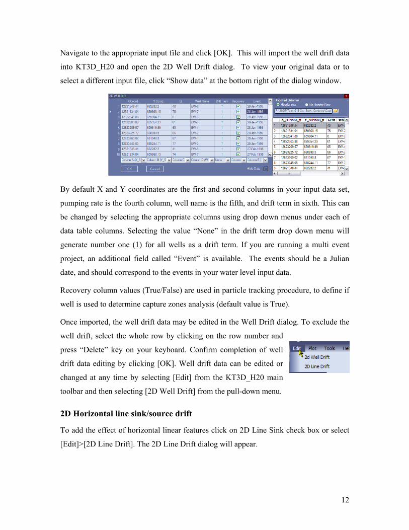
Navigate to the appropriate input file and click [OK]. This will import the well drift data
into KT3D_H20 and open the 2D Well Drift dialog. To view your original data or to
select a different input file, click “Show data” at the bottom right of the dialog window.
By default X and Y coordinates are the first and second columns in your input data set,
pumping rate is the fourth column, well name is the fifth, and drift term in sixth. This can
be changed by selecting the appropriate columns using drop down menus under each of
data table columns. Selecting the value “None” in the drift term drop down menu will
generate number one (1) for all wells as a drift term. If you are running a multi event
project, an additional field called “Event” is available. The events should be a Julian
date, and should correspond to the events in your water level input data.
Recovery column values (True/False) are used in particle tracking procedure, to define if
well is used to determine capture zones analysis (default value is True).
Once imported, the well drift data may be edited in the Well Drift dialog. To exclude the
well drift, select the whole row by clicking on the row number and
press “Delete” key on your keyboard. Confirm completion of well
drift data editing by clicking [OK]. Well drift data can be edited or
changed at any time by selecting [Edit] from the KT3D_H20 main
toolbar and then selecting [2D Well Drift] from the pull-down menu.
2D Horizontal line sink/source drift
To add the effect of horizontal linear features click on 2D Line Sink check box or select
[Edit]>[2D Line Drift]. The 2D Line Drift dialog will appear.

13
Click the [Show Data] button to open the data import dialog. Choose the appropriate
input file and click [OK]. The table to the left of the dialog will fill in with the input data.
Select the appropriate columns for coordinates, drift term, and head. Note that Drift Term
and Head must be numeric values, and there is no event date column. Single imported
data set will be used for all kriged events.
Click [OK] to confirm completion.
2D Circular pond
Two dimensional circular pond drift can be added by clicking on 2D Circular Pond check
box or select [Edit]>[2D Pond Drift]. The 2D Pond Drift dialog will appear.
Click the [Show Data] button to open the data import dialog. Choose the appropriate
input file and click [OK]. The table to the left of the dialog will fill in with the input data.
Select the appropriate columns for coordinates, radius, strength and drift term. [OK] to
confirm completion.

14
Setting variogram parameters
At the {Variograms} tab, the user can set and view variogram parameters. In this version
of KT3D_H2O only one variogram at a time may be selected. (This differs from original
GSLIB KT3D which accepts “unlimited” number of variograms. For the detailed
explanation of variogram parameters please refer to the GSLIB Book.
For variogram modeling, KT3D_H2O uses
the GSLIB programs “gamv” and “vmodel”.
To model single the variogram, click on the
[Variogram Model] button which opens
variogram dialog on variogram modeling
page. In case of multi event projects there are
two options to model variogram: The first
option is to run Variogram model using all
data as a one data set and the second options
is run Variogram model using each event as a
separate data set. The Event Selector dialog
will appear. Select the appropriate events and
click [OK].
The UI automatically calculates the
experimental variogram(s) model (using “gamv”) and plots them on variogram plot as a
blue line(s)).

15
Range
Sill
Nugget
Model Curve
Experimental Varigram CurvesVaria
nce
Con
tibut
ion
After adjusting model parameters it is necessary to click on [Apply] button to recalculate
model (using GSLIB “vmodel” program) and refresh the plot. At any time you can switch
to the experimental page and adjust experimental parameters. After parameters are
adjusted click on [Apply] to execute “gamv” program and refresh the variogram plot.
After the appropriate parameters are entered and “best fit” is achieved, click the [OK]
button to return to variogram page.

16
Running the Kriging
Before kriging, it is recommended that you save your MapWindow project file and your
KT3D parameter file. To execute the KT3D kriging program click the button.
You can terminate kriging at any time by pressing the [ESC] key.
Single event kriging
To run kriging, click the button. After kriging is finished, the UI will prompt
you to enter an ASCII grid file name. The grid will be saved in the same directory as the
.xpar or .xpars file and imported to the MapWindow project map. MapWindow
automatically generates a *.bmp file for viewing purposes and an *.mwleg file, which is
XML file that contains layer legend information. KT3D_H2O also generates an XML file
(*.xasc) which contains all parameters and all input data used for the kriging. Data from
XML file can be imported at any time selecting the [File]-[Import]-[Xml Data].
To generate contours select [Plot] then [Contours]. A file selection dialog will appear.
Select the appropriate grid file and click [OK].
The “Generate Contours” dialog will appear.
Contours levels may be set two ways. Fist, you
may set the maximum and minimum values and
contour interval. By default, the maximum and
minimum contour values are determined from the
grid, but these values may also be entered
manually. Second, you may specify levels by
entering level values separated by a single space in the text box. After you have
determined the contour levels, click the [Generate] button. This will generate a shapefile
(.shp) showing the contours. You will be prompted for the shapefile name, and the
location where the file will be saved. By default, this is the project directory. Once you
click [Save] the shapefile will be displayed in the MapWindow project.

17
Multi Event kriging
To run kriging, click the button. The Event
Selector dialog will appear. Select the appropriate events
and click [OK]. After each event is kriged you will be
prompted to enter the ASCII grid file name. To avoid
repeating this step, click on [Tools]-[Project Settings], then
check “Overwrite Existing Files”. If this option is selected,
the UI will generate and use default ASCII grid filenames
and save them in the project directory. The default file
name is constructed as: project file name + “_” + event date
(for example, “newproject_28-Jan-1998.asc”). All kriged
grids will be added to the project map. If you don’t want your kriging grid files to be
added to the map, click [Tools]-[Project Settings] and uncheck “Add Results to Map”. It
may be necessary to do this if you have a large number of kriging events because plotting
each map can significantly slow down your system.
To generate contours in multi event projects, select [Plot]-[Contours]. The Event Selector
dialog will appear. Next to the Event is the column “GridFile” populated with the default
equivalent ASCII grid file name. If the ASCII file name or directory was anything other
than the default assigned by the UI, then it is necessary to select the grid file manually.
To do this, right click in the event “GridFile” cell. You will be prompted to select
another ASCII grid file which will be used for contouring in that Event.
Select desired events and click [OK]. Contour shapefiles will be created for each event.
See Single Event Contouring for a full description of the contouring process.
Kriging output results also can be viewed by plotting nodal values, Select [Plot] then
[Kriged Nodal Values], select event and UI will generate point shape file with X and Y
coordinate, row, column and kriged value at every node of your grid.

18
Exporting kriging results
Kriging results can be exported as a binary file (*.kbf). To do that select [File]-[Export]-
[KT3D_H2O Binary file] (for file format see Appendix B). Then in “file type” dropdown
menu select “KT3D_H2O Kriging Binary File (*.kbf)”. Enter the file name. For Multi
Event projects, the Event Selector Dialog will appear. Select event grid files you wish to
export.
To export kriging results as a Surfer ASCII grid file select [File]-[Export]-[ASCII Surfer
Grid]. For a Multi Event project, the Event selector dialog box will appear. Select the
Event grid files you wish to export. For each event you will be prompted to enter the
Surfer ASCII grid file name and location. To skip this step, click on [Tools- Project
Settings] then check “Overwrite Existing Files”. If this option is selected, the UI will
generate and use default Surfer grid filenames and save them in the project directory. The
default file name is constructed as: project file name + “_” + event date (for example,
“newproject_28-Jan-1998.grd”). Surfer grid files can also be automatically generated
during Multi Event kriging. To do this, go to the {Multi Event} tab, check “Generate
Surfer grid file during multi-event run”. Note this option must be selected before kriging
is performed.
Importing kriging results
Kriging results can be imported at any
time by selecting [Plot]-[Color Flood]. For
Mulit-Event projects, a “Event Selector”
dialog will appear. If all files have
default file names, the “Gridfile” cell next
to each event will be populated with the
corresponding ASCII grid file name
(*.asc). Alternately, you can select any
ASCII grid file to plot by right-clicking in
the “Gridfile” cell next to the Event. A file selector dialog will appear. Choose the
appropriate grid file (*.asc) and click [Open].
19
To import kriging results from a kriging binary file, click on “Import from Binary File”
checkbox then from File open dialog select “Kriging binary
file”. The UI will read all saved events in the binary file, the Event selector dialog will
appear. Select which events to plot. This will generate new ACII grid files for each
selected event. You will be prompted to enter a file name for each. To skip this step,
before importing the binary file, click on [Tools]-[Project Settings] in the main
KT3D_H20 window. then check “Overwrite Existing Files”. If this option has been
selected when the binary file is imported, the UI will generate and use default ASCII grid
filenames for each event and save them in the project directory. The default file name is
constructed as: project file name + “_” + event date (for example, “newproject_28-Jan-
1998.asc”).

20
Append new Events
To append a new sampling event(s) to an existing Project data set, click [Tools]>[Append
Data] then select the appropriate dataset to append. In the dialog form select appropriate
columns as explained in the “Importing Data” section. To confirm that your new data set
is imported correctly, click [OK]. The new data will be appended to the end of the data
table.

21
Particle tracking
The grids generated as described in the previous section can now be used to generate a
particle tracks. Particle tracking is performed in
KT3D_H2O using TransientTracker (Attachment
2). It supports the approximate evaluations of
historic and future contaminant migration; of
hydraulic capture zones developed by pump-and-
treat type remedies; and other analyses that benefit
from the ability to track particles on a surface. The
particle tracking utility has been adapted to use the
program TransientTracker as a processing engine
while KT3D_H2O is used to generate ASCII input
files and for post-processing TransientTracker
outputs.
All particle tracking settings are in the {Part.Track} tab. Here you can set particle starting
locations, tracking type, tracking parameters and output type.
Setting particle tracking parameters
The following parameters are required to perform particle tracking:
Input type format Hydraulic Conductivity in Aquifer Entered as single numeric value in GUI
Porosity in Aquifer Entered as single numeric value in GUI
Starting locations of particles
May be specified in using GUI as described; or imported from an external file. Supported file types:
Microsoft Excel ,or ASCII text including XY coordinates of each starting location; or an ESRI shapefile (.shp)
showing all starting locations.
Results of KT3D water level kriging
.asc files generated by KT3D. When KT3D is run, these files are saved automatically in the same
directory as the .xpar or .xpars file, and are imported automatically before particle tracking is run.
For practical reasons all input parameters which contain a time component must use the
unit “days”.

22
For explanation particle tracking parameters please refer to the included Transient
Tracker documentation (Attachment 2).
Setting particle starting locations
There are five options to generate particle starting locations:
a. Read from File: To import starting locations from a file, under the {Part.
Tab}, click button to expand the KT3D_H2O main window. Then click
Open file button next to “Start. Loc File”.
Select the type of input file
(ASCII, Excel or Shapefile). After data are imported, use column selector dropdowns to
select column for X and Y coordinate.
b. Automated: For projects using a 2D well drift, there is an option to
generate particles around each well in circular envelopes. Enter the number of particles
per envelope, number of envelopes, and radius of envelopes.
For example, if the radius of the first envelope is 50 ft, then the
radius of the second is 100; the radius of the third envelope is
150 ft, and so on. This option can be executed only using
backward tracking.

23
c. Custom: This option allows you to generate particle starting locations by
drawing polylines or polygons, or by selecting shapes from existing polygon shape files.
To open the Custom Particles dialog, select “Custom” from the pull-down menu next to
“Starting Loc”.
1. To draw a
polyline: Select the {polyline}
tab on dialog menu. In the
Project Map, left click to begin the
line, and right click to end it. In the
Custom Particles dialog, type in the
desired number of particles per
segment. The total number of
particles will be calculated based on the number of segments in the polyline and the
number of particles per segment. After you have drawn the polyline and set the number
of particles per segment, click [Add Particles]. Red dots will be converted to blue,
indicating that those locations are saved in memory. To add more particles simply draw
another polyline.
2. To draw a polygon: From the Custom Particles toolbar select the shape
of polygon (irregular, n- sided regular or rectangular). Left click to start the polygon and
right click to end it. To draw a square, select the rectangle tool and hold down the Ctrl
key while drawing the rectangle. Particles may be generated inside the polygon one of
two ways: either enter the number of
particles next to “# of Particles”, which will
generate the set number of particles at
random locations inside the polygon; or
check “Use Grid Nodes” to generate
particles at all kriging grid nodes inside the
polygon.

24
To use existing polygon shape file: In the Custom Particles dialog, select the shapefile
import tab from the dialog toolbar . Select the polygon shape file from the legend
then select desired shape. Enter number of particles as explained in section 2 above and
click [Add Particles].
To generate a point shapefile from generated particle locations, click [Create Shape File].
After generating particles click [OK]. The UI will populate a particle worksheet with
particle coordinates.
d. Custom Regular Grid: Select “Custom Regular Grid”
from the pull-down menu next to “Starting Loc. Options”. Enter X and
Y coordinates and cell size. Default values are grid extents used in the
kriging.
e. Quick “screen” particle tracking: For
single event projects, hold down the Shift key (cursor will
change to the target shape) and click with right mouse
button at the particle starting location on the map. The
program will instantly run particle tracking using existing
particle tracking parameters. For Multi-Event projects, this
option is only available using transient tracking. In the
{Part. Track} tab, select “Transient Tracker”. As with
single-even projects, hold down the shift key and right click
on the starting location on the map. The event selector dialog will appear. Select the
grids to be used in transient tracking. The particle will be tracked along the selected grids
according to the specified step size until the last date in the Event Selector Dialog (“End
Time for Transient Tracker”). By default, this is the current date. More information on
transient tracking is available in the attached Transient Tracker documentation
(Attachment 2).

25
Running particle tracking
1. To run particle tracking for a single event project: set up particle starting
locations as described in the previous section. Select particle tracking shapefile output
type (point or polyline) and define particle tracking parameters. Then from the
Mapwindow legend, select kriged grid file. In the main KT3D_H20 toolbar, click the
“Run Part. Track” button. . After tracking is finished, you will be prompted
to enter the path and output shapefile name. The output shapefile will be saved in the
specified directory and added to the project map. Note: the grid you selected before
running particle tracking the first time will remain active until you select a new grid.
There is no need to select the grid each time you run particle tracking.
2. Multi event project
Two types of tracking are available for Multi Event projects: Multi
event and Transient tracking.
Multi Event: In the {Part. Track} tab, under “Tracking Type”
select “Multi-Event”. Define particle tracking parameters and click the “Run Part. Track”
button. The Event Selector dialog will appear. Select the appropriate event grid files and
click [OK]. KT3D_H2O will perform particle tracking on each grid file individually
using the specified particle tracking parameters for each event and also output files will
be generated for each event.
• Transient Tracker: In the
{Part. Track} tab, under “Tracking
Type” select “Transient Tracker”.
Define particle tracking parameters
and click the “Run Part. Track”
button . The Event
Selector dialog will appear. The
column “GridFile” is populated
with the corresponding event

26
default ASCII grid file names, any grid files may be selected by right clicking on the
event GridFile cell. Check the appropriate events kriged grid files. The bottom of the
Event Selector dialog contains an event called “End Time for Transient Tracker”. Enter
the date that transient tracking stops. By default, this is the current date. This date may
be changed manually, or may be chosen from the calendar. To view the calendar click
slowly two times on the “End Time for Transient Tracker” Event Date cell. Transient
tracking will be performed along the selected grids from the first date selected to the
specified end date. Step size must be specified in the particle tracking parameters, and
must be in units of “days”. For more information on the transient tracking process, see
the attached Transient Tracker documentation (Attachment 2).

27
Hydraulic Capture Zone analysis
Hydraulic Capture Zone analysis records the fate of particles during tracking simulation.
TransientTracker (Attachment 2) includes functionality for removing particles at the
margins of the grid domain; at stagnation zones; at sinks when forward tracking. The
program records the fate of particles in an ASCII summary file. The contents of this file
is used by KT3D_H2O to illustrate capture zones. This section describes how to use
KT3D_H2O to generate capture zone maps and capture frequency maps.
• Hydraulic capture zones: In the {Part. Track} tab under “Starting Loc. Options,
select “Custom regular grid” and under “Tracking Type” select Multi Event Tracker”.
Define particle tracking parameters and click “Run Part.Track” button .
After particle tracking is finished, a capture ASCII grid file is generated. This file
contains an array of integers which represents the different extraction wells, boundaries,
and other types of zones, or sinks where a particle was removed from particle tracking.
KT3D_H2O converts those integers into zone an explanation shown in the MapWindow
28
legend. By default particle pathlines shapefiles are not generated during hydraulic capture
analysis. This option can be selected by checking the “Generate Particle Tracking
Shapefiles” box in the {Part. Track} tab .
• Capture Frequency map: For Multi Event projects, there is an additional option
to calculate a capture frequency map. This map describes the number of times a particle
was removed at an extraction well compared to the number of events calculated (i.e., the
fraction of capture for each particle). For example, frequency of 0.5 indicates that during
all the events for which capture zones were calculated, the particle was captured by an
extraction well 50% of the time. This suggests that on the basis of the measured water
levels, the assumed measurement errors, and the linear-log drift gridding approach
employed, a particle originating from the given location would be captured by the
combined pumping of extraction wells about 50 percent of the time. Hence, these maps
illustrate the relative frequency with which particles of groundwater are captured under
the varying conditions represented by different water level events.
A capture frequency map may be generated two ways. First, it will be generated
automatically at the end of a capture zone analysis. After tracking has been completed
for all events, a prompt will appear asking if you want to save the capture frequency map.
Specify the path and file name and click “Save”. Second, a capture frequency map may
be created from the combination of any capture grid files. Select [Plot]-[Frequency Map]
then select desired capture zone analysis gridfiles. Specify the path and file name and
click “Save”. The capture frequency map will be automatically added to the
MapWindow project map.
Exporting Hydraulic Capture Zone analysis results
Capture Zone analysis results can be exported and saved as a binary file (*.cbf) (for file
format see Appendix B). To do that select [File]-[Export]-[KT3D_H2O Binary file].
Then, in file type dropdown menu, select “KT3D_H2O Capture Binary File (*.cbf)”.
Enter the file name. For Multi Event projects, the in the Event Selector dialog box will
appear. Select the event capture grid files you wish to export.

29
References
Deutsch, C., and Journel, A., (1992). GSLIB: Geostatistical Software Library and User's
Guide. Oxford University Press, 340 pp.
Tonkin, Matthew J., and Larson, Steven P., 2002. "Kriging Water Levels with a
Regional-linear and Point-logarithmic Drift". Ground Water, March/April 2002.
MAP WINDOW Desktop User Guide. http://www.mapwindow.org/wiki/index.php/MapWindow:Desktop

30
Appendix A
KT3D_H2O Input Formats
KT3D_H2O supports importing data from Microsoft Excel versions 2000-2007 (*.xls,
*.xlsx, *. xlsb and *.xlsm) files, Microsoft Access versions 2000-2007 (*.mdb and
*.accdb) files, ESRI Shape Files (*.shp) and ASCII (.txt or .dat) files with values
separated by space, comma or tab.
Water Level data
KT3D_H2O required following set of variables in input data:
First line is assumed to be header line for example:
“X Y WL WellIDDate” then for each measurement line with XC(i), YC(i),
Value(i), OID(i), Event(i)
Variables
1 Header Line
2 XC(i), YC(i), Value(i), OID(i), Event(i)
Where this line is repeated n measurements times.
The table below provides explanation of the variables used in KT3D_H2O input data.
XC(i) X coordinate of the object (i)
YC(i) Y coordinate of the object (i)
Value(i) Kriging variable (i)
OID(i) Name of the object (i)
Event(i) Date of the event (Required for Multi Event projects)

31
By default, KT3D_H2O assigns the first column in your input data as X coordinate,
second as Y coordinate, third as kriging variable and fourth as an object name. Any input
option column reference can be changed using the drop down menus. For multi-event
projects, a fifth variable, “Event” is required in format of Julian date (for example
01/01/2004).
Well drift data
Data defining locations and characteristics of each well used as a well drift should be
provided in following format
Variables
1 Header Line
2 qxx(i), qyy(i), qqq(i), idtwell(i), qdrift(i), qtype(i), wellname(i), qevent(i) where this line is repeated nwells times.
The parameters listed above have the following definitions.
NWELLS KT3D_H2O will read file to the end, so no need to specify the number of wells. Lines begin with character “#” are considered as comment lines.
qxx(i) X –coordinate of the well i
qyy(i) Y –coordinate of the well i
qqq(i) Pumping rate of the well i for the current event
wellname(i) A name for the well
qdrift(i) Drift term for well i
qtype(i) -- Specify the well as recovery (R) or not recovery (N) Used in capture zone analysis.
qevent(i) Event Date in format of Julian date Line Drift Data
LINEFILES(i): These files define the locations and characteristics of sink line segments.
They are simple ASCII files and provide information in the following format.

32
Variables
1 Header Line
2 lxs(i),lys(i),lind(i),lval(i) where this line is repeated NLIN times.
The parameters listed above have the following definitions.
Lx(i) -- X location of point(s) i
Ly(i)-- Y location of point(s) i
Ldrift(i) -- Indicator of line sink/source drift term
Lval(i) -- Head value for the line feature.
Levent(i)-- Event date in format of Julian Date
Pond Drift Data
Pond Drift File: This file defines the locations and characteristics of circular and should
be provided in the following format.
Variables
1 Header Line
2 pX(i),pY(i),pRadius(i),pStrenght(i),pDrift where this line is repeated by number of ponds.
The parameters listed above have the following definitions.
pX(i) Pond center X coordinate
pY(i) Pond center Y coordinate
pR(i) Pond Radius
pStrenght(i) Pond Strength
pDrift(i) Indicator of pond drift term For detailed information about each input parameter please refer to the Attachment 1.

33
Appendix B Binary File Formats
Kriging Binary file (*.kbf) and Capture Binary file (*.cbf) have identical structure, for the
practical reasons they have different extensions. Binary file has one header section and
“unlimited” grid array sections.
Data types used in binary files:
Type Description long 32 bit signed integer double 64 bit double precision floating point value Text 1 bit
Header section describes dimension of 3D array and contains all the data for defining the
grid
Element Type Description nLay long number of layers in the grid (nlay=1) nRow long number of rows in the grid nCol long number of columns in the grid xLL double X coordinate of the lower left corner
of the grid yLL double Y coordinate of the lower left corner
of the grid Rotation double not currently used BlankValue double nodes are blanked if equal to this valueTxt Text Some file description 50 characters
long. xSize(ncol-1) double One dimensional array representing
spacing between adjacent nodes in the X direction (between columns)
ySize(nRow-1) double One dimensional array representing spacing between adjacent nodes in the Y direction (between rows)
34
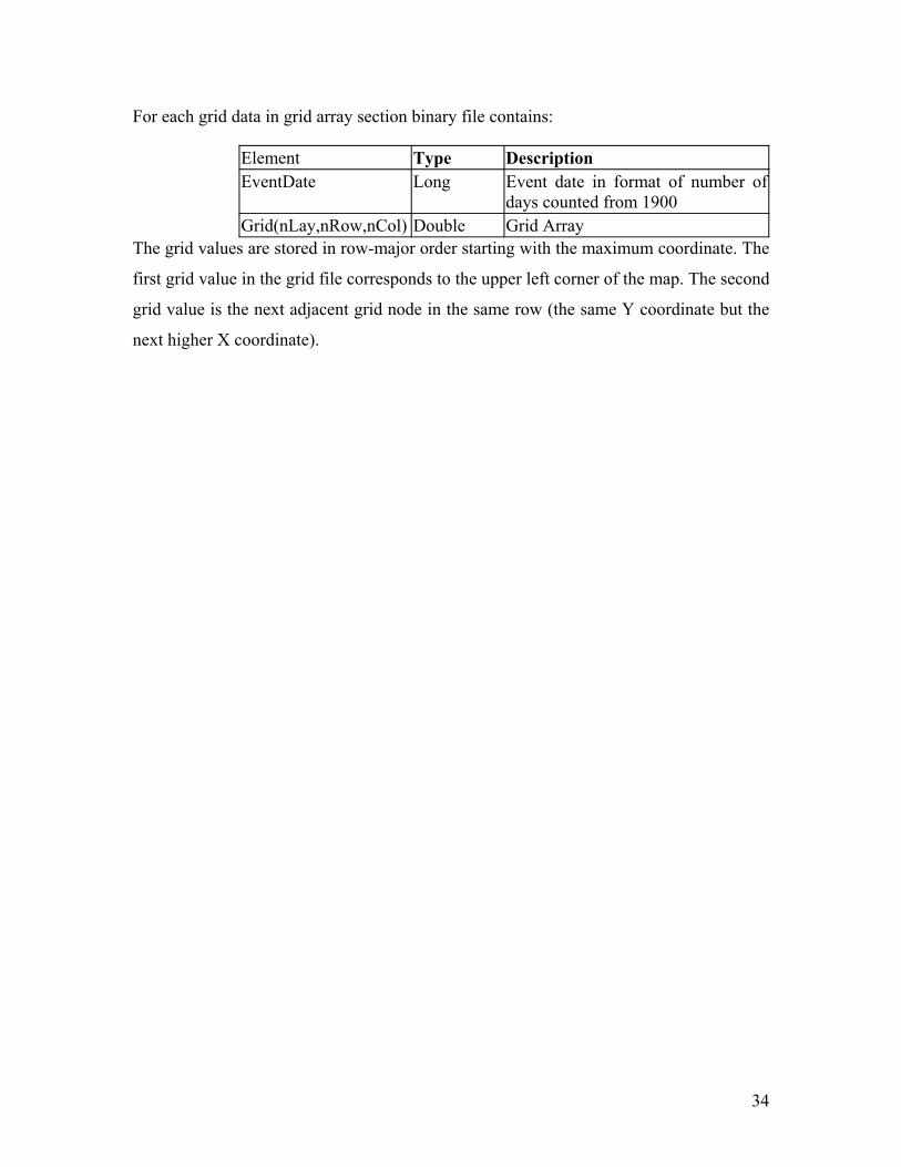
For each grid data in grid array section binary file contains:
Element Type Description EventDate Long Event date in format of number of
days counted from 1900 Grid(nLay,nRow,nCol) Double Grid Array
The grid values are stored in row-major order starting with the maximum coordinate. The
first grid value in the grid file corresponds to the upper left corner of the map. The second
grid value is the next adjacent grid node in the same row (the same Y coordinate but the
next higher X coordinate).

35
Appendix C ArcInfo ASCII Grid Files Formats
ArcInfo ASCII Grid files [*.asc] contain seven header lines that provide information
about the size and limits of the grid, followed by a list of Z values. The fields within
ASCII grid files must be space delimited.
The listing of Z values follows the header information in the file. The Z values are stored
in row-major order starting with the maximum Y coordinate. The first Z value in the grid
file corresponds to the upper left corner of the map. The second Z value is the next
adjacent grid node in the same row (the same Y coordinate but the next higher X
coordinate). When the maximum X value is reached in the row, the list of Z values
continues with the next higher row, until all the rows of Z values have been included.
The general format of an ASCII grid file is:
Element Description ncols ncol number of columns in the grid nrows nrow number of rows in the grid xllcenter X X coordinate of the lower left center of the grid
cell yllcorner Y Y coordinate of the lower left center of the grid
cell dx xsize Grid cells size in X direction dy ysize Grid cells size in Y direction Nodata_Value Nodata nodes are blanked if equal to this value Grid(nRow,nCol) Grid Array
The grid values are stored in row-major order starting with the maximum coordinate. The
first grid value in the grid file corresponds to the upper left corner of the map. The second
grid value is the next adjacent grid node in the same row (the same Y coordinate but the
next higher X coordinate).
Attachment 1 KT3D_H2O v3.0 A Program for Kriging Water Level Data using Hydrologic Drift Terms Theoretical Documentation

KT3D_H2O v3.0
A Program for Kriging Water Level Data
using Hydrologic Drift Terms
Theoretical Documentation

DESCRIPTION OF THE KT3D_H2O PROGRAM SUITE
OUTLINE ...................................................................................................................................... 4
BACKGROUND ........................................................................................................................... 5
UNIVERSAL KRIGING.............................................................................................................. 5
GSLIB......................................................................................................................................... 8
ADDITIONAL DRIFT TERMS IMPLEMENTED IN KT3D_H2O....................................... 9
1. POINT SINK OR SOURCE OF KNOWN STRENGTH ....................................................................... 9
2. HORIZONTAL LINE SINK OR SOURCE OF KNOWN STRENGTH ................................................. 10
3. CIRCULAR LEAKING POND OF KNOWN STRENGTH................................................................. 11
KT3D_H2O PROGRAM INPUTS............................................................................................ 13
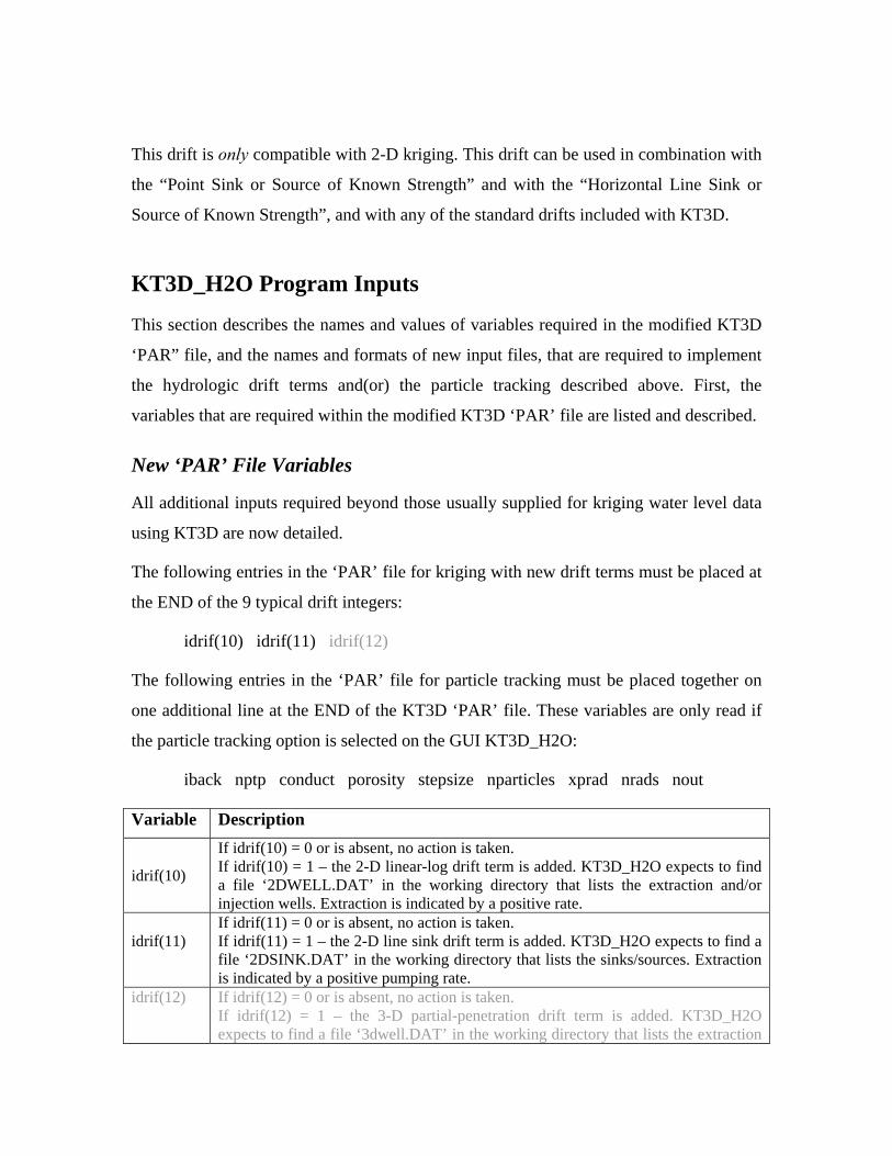
NEW ‘PAR’ FILE VARIABLES .................................................................................................... 13
POINT SINK OR SOURCE OF KNOWN STRENGTH ......................................................................... 14
HORIZONTAL LINE SINK OR SOURCE OF KNOWN STRENGTH ..................................................... 15
EXAMPLE DATA SETS ........................................................................................................... 17
[NOTE: EXAMPLES TO BE CONVERTED TO BE USED IN KT3D_H2O GUI VERSION
3.0] ................................................................................................................................................ 17
POINT SINK OR SOURCE OF KNOWN STRENGTH ......................................................................... 17
HORIZONTAL LINE SINK OR SOURCE OF KNOWN STRENGTH ..................................................... 18
CIRCULAR LEAKING POND OF KNOWN STRENGTH..................................................................... 20
ACKNOWLEDGEMENTS ....................................................................................................... 21
ACKNOWLEDGEMENTS ....................................................................................................... 22
TECHNICAL SUPPORT........................................................................................................... 22
FREQUENTLY ASKED QUESTIONS.................................................................................... 22
REFERENCES............................................................................................................................ 25

APPENDIX A: KRIGING WATER LEVELS WITH A REGIONAL-LINEAR AND
POINT-LOGARITHMIC DRIFT, GROUND WATER, 2002............................................... 27
Outline
This document describes the KT3D_H2O v2.0 programs which provide a customized
version of the popular kriging program KT3D (Deutsch and Journel, 1992) that has been
modified to include drift terms derived from the hydrologic sciences. These drift terms
are included in order to account for the influence of point, line and circular boundaries
such as wells, trenches, rivers and ponds, when kriging groundwater level data. Use of
the KT3D_H2O programs should always be accompanied by review of the
documentation for KT3D provided in the GSLIB book (Deutsch and Journel, 1992).
Background
Though kriging is widely used for constructing gridded datasets suitable for contouring,
when kriging water levels in the vicinity of pumping wells, rivers and trenches, large
departures from the underlying trend are evident that correlate with areas of drawdown or
mounding, and that render the maps aesthetically displeasing and illustrate weaknesses in
the interpretation of the data. The methods incorporated in the KT3D_H2O programs
mitigate some of these weaknesses, by including information in the kriging process to
account for these features. This information is included through the description of an
assumed underlying trend in the data. In this document the term drift is used
synonymously with the term trend, to describe a pattern that has a deterministic source or
can be approximated by deterministic means. Since the method is based on automated
gridding, it can be more consistent between data sets and between analysts than methods
based on hand contouring. Since the method is based on Universal Kriging, a brief
overview of Universal Kriging is provided first.
Universal Kriging
Kriging is employed in the hydrologic disciplines for interpolating measured data to
regular grids suitable for contouring. One advantage of kriging over other interpolation
methods is that, in the absence of measurement error or replicates (co-located data), it is
an exact interpolator. Chiles and Delfiner (1999) provide a detailed summary of kriging.
Two popular forms of kriging employed for interpolating real-valued data are (1) simple
kriging and (2) ordinary kriging. In simple kriging, the mean of the data, m, is assumed
to be constant everywhere and its value known a-priori. In ordinary kriging the mean is
assumed to be unknown a-priori, and is estimated using either all or some local (moving)
neighborhood of the measured data. The methods described in this discussion are based
upon ordinary kriging. In the most common implementation of ordinary kriging, the
mean is assumed to be constant and equivalent to the mean of the data – that is, m = m(x).
However, ordinary kriging can support a spatially varying mean which is commonly
described as a smoothly-varying mean or “drift.” When a spatially varying mean is

incorporated, the kriging estimate can be illustrated as the sum of two components, the
mean and a zero-mean residual:
H(x) = m(x) + ε(x) (1)
Where:
H(x) = the kriging estimate
m(x) = the smoothly-varying trend or drift
ε(x) = the zero-mean random residual from the drift
This approach is commonly referred to as Universal Kriging (UK). This trend is usually a
simple function of the spatial coordinates, such as a linear or quadratic function of the
data X and Y coordinates. However, the kriging formulism is not limited to this form of
drift, and is generally only limited to drift functions that can be fit through the solution of
the (linear) system of kriging equations. For discussion on the use of trends in kriging
refer to Volpi and Gambolatti (1978).
Kriging with a linear trend model or drift is available through popular programs such as
Surfer® and TecPlot®. A linear drift is suitable in situations where unidirectional regional
groundwater flow exists, a condition often encountered. The UK estimator for gridding
water level data using this approach can be illustrated as:
H(x,y) = A + BX + CY + ε(x,y) (2)
Where:
H(x,y) = the estimated elevation at location (X,Y)
X = the easting or X ordinate
Y = the northing or Y ordinate
A, B, C = coefficients for the plane fitting the groundwater heads
ε (x,y) = the residual from the drift
The linear drift may not be suitable in areas (a) where singularities occur within the data
field such as created by pumping wells, (b) where lateral hydrologic boundaries such as
the lateral termination of aquifer materials are present, (c) where there is a significant
vertical component of flow, and/or (d) where there are substantial changes in aquifer

properties or preferential pathways. If these effects can be represented in the trend using
appropriate functions with linear coefficients, these difficulties can be resolved and
kriging can produce suitable maps. Tonkin and Larson (2002) and Brochu and Marcotte
(2003) describe the incorporation of analytic elements within the kriging method to
account for effects due to pumped wells and boundaries.
By way of example: when kriging water level data in the presence of significant
groundwater extraction or injection, the residuals (the difference between the measured
data and the fitted drift surface) arising from the use of a linear drift typically indicate
large local departures from the drift in the vicinity of the wells that correlate with areas of
drawdown (or mounding in the case of injection wells). The use of drift terms in
universal kriging based on hydrologic principals – such as drawdown in response to
pumping – can improve the inference that can be drawn from measured water level data.
This is illustrated in plan (Figure 1) and cross-section views (Figure 2). This is because
the component of spatial correlation in the water levels that results from the influence of
the boundary is explicitly included in the drift. Hence residuals are typically smaller
when an appropriate drift is used. This ensures that a smaller proportion of the spatial
covariance (or correlation) must be explained through the use of a variogram, the proper
estimation of which might require much more data than are available. The incorporation
of drift terms based on hydrologic principles is described in Tonkin and Larson (2002)
and Brochu and Marcotte (2003).

GSLIB
GSLIB is an acronym for Geostatistical Software LIBrary, referring to a collection of
geo-statistical programs developed at Stanford University. One of these programs is
KT3D, a general program for point or block kriging in two or three dimensions. The
GSLIB programs are fully described in Deutsch and Journel (1998). KT3D_H2O is based
upon KT3D. It is strongly recommended that users of the KT3D_H2O programs obtain a
copy of Deutsch and Journel (1998) both for the theoretical discussions of geo-statistics
provided therein, and for the detailed descriptions of the input files required and output
files produced by the KT3D program. Details of these input and output files are not
Figure 1 Plan View Comparison of Water Levels Kriged Excluding and
Including Pumping Well Drift Term
Figure 2 Section View of Water Levels from Above Kriging Example

provided in this documentation. However, the section “KT3D_H2O Program Inputs”
described additional inputs that are required, beyond the standard KT3D inputs. In
particular, KT3D uses an integer array (IDRF) to indicate which drifts are to be included
in the kriging. The standard KT3D IDRF array includes nine integers, for the nine drifts
available. The additional drifts added to KT3D_H2O are implemented by extending this
IDRF array to include – presently – 13 integers, for the nine original drifts plus four
additional drifts.
No options available to KT3D have been disabled to make KT3D_H2O. Array size
limitations as listed by the dimensions in the ‘KT3D.INC’ file provided with GSLIB are
adhered to in compiling KT3D_H2O. Significant arrays added to KT3D_H2O in adding
the kriging and particle tracking functionality are allocatable, however, and should not be
exceeded unless the program encounters problems allocating the memory. KT3D_H2O is
compiled in single precision to reduce memory requirements. In several tests, comparison
of grids and particle tracks calculated using single precision and double precision codes
showed no noticeable improvement using double precision. However, if you encounter
unsatisfactory results that may be linked to precision – in particular, if you encounter
problems with particle tracking that could not be improved by modifying input options - a
double-precision compiled version of the code can be provided upon request.
Additional Drift Terms Implemented in KT3D_H2O
Presently, four drift terms have been added to KT3D_H2O, beyond those included in the
original KT3D program. Three of these drifts are only compatible with kriging of water
levels in two dimensions (2-D). One of these drifts is compatible with kriging of water
levels in 3-D. The first of these drifts to be developed, the “linear-log” drift, is described
first. Subsequently the additional drift terms are described. Inputs required to implement
each boundary drift term are described in the section “KT3D_H2O Program Inputs”.
1. Point Sink or Source of Known Strength
This drift was added to account for mounding (or drawdown) in response to injection (or
extraction) at a known rate at one or more wells. For a single well, the Thiem equation
states that, for consistent units:

⎟⎠⎞
⎜⎝⎛=
rR
TQsr 10log
23.2π
(3)
Where:
r = radial distance from the pumped well
R = radius of influence
sr = drawdown due to pumping
Q = pumping rate
T = aquifer transmissivity
Examination of (3) indicates that pumping at a single well produces a logarithmic pattern
of drawdown centered on the pumping well. Under certain assumptions, superposition
can be used to sum the effect of multiple extracting or injecting wells. This essential
information can be distilled and combined with the linear drift shown in (2) to give:
H(x,y) = A + BX + CY + Dn
1Σ Qilog10(ri) + ε (x,y) (4)
Where:
Qilog10(ri) = drawdown factor due to pumping at the ith well
D = the linear regression coefficient for the drawdown factors n
1Σ = the summation from 1 to n where n = the number of pumped wells
A full derivation of (4) is given in Tonkin and Larson (2002). This drift term can be used
in combination with any of the standard two-dimensional drifts included with KT3D.
2. Horizontal Line Sink or Source of Known Strength
This drift was added to account for mounding (or drawdown) in response to horizontal
linear features of known extraction (injection) rate, such as interception trenches or
infiltration galleries. This implementation is based on the Analytic Element Method
(AEM) described by Strack (1989) and further documented and incorporated into the
AEM program TWODAN (Fitts, 2004). The complex potential representing a line sink is:
( ))1()1()1()1(4
−−−++=Ω ZLnZZLnZπLσ (5)

)12()21(2
zzzzzZ
−+−
= (6)
Where:
L = the length of the line sink/source
Z = a dimensionless complex variable
(z1, z2) are the complex coordinates of the ends of the line
z = x + iy is the point where Z and Ω are evaluated
Since σL, the discharge-per-unit-length is known out the outset then solving for Ω is a
linear problem that can be included in the linear kriging system of equations. This
essential information can be distilled and combined with the linear and logarithmic drifts
shown in (4) to give:
H(x,y) = A + BX + CY + Dn
1Σ Qilog10(ri) + E
m
1Σ L(ri) + ε(x,y) (7)
Where:
L(ri) = drawdown factor due to effects of the ith line sink
E = the linear regression coefficient for the line sink factors m
1Σ = the summation from 1 to m where m = the number of line sinks
This drift is only compatible with 2-D kriging. This drift can be used in combination with
the “Point Sink or Source of Known Strength”, and with any of the standard 2D drifts
included with KT3D.
3. Circular Leaking Pond of Known Strength
This drift was added to account for the potentiometric response of a water table
(unconfined) aquifer to infiltration through the base of a circular pond. The approach is
based on the Analytic Element Method (AEM) described by Strack (1989). For a circular
pond of radius R this can be represented by the following schematic and equations:

Within the element:
(0 ≤ r1 ≤ R) ( ) ( )[ ]221
2111p 4
1 R) ,y , xy, (x,G Ryyxx +−+−−= (8)
Outside the element:
(R ≤ r1 < ∞) ( ) ( )2
21
21
2
11p 4 R) ,y , xy, (x,G
RyyxxLnR −+−
−= (9)
This essential information can be distilled and combined with the linear, logarithmic and
line sink/source drifts shown in (7) to give:
H(x,y) = A + BX + CY + Dn
1Σ Qilog10(ri) + E
m
1Σ L(ri) + F
o
1Σ P(ri) + ε(x,y) (10)
Where:
P(ri) = mounding factor due to effects of the ith leaking pond feature
F = the linear regression coefficient for the leaking pond features o
1Σ = the summation from 1 to o where o = the number of pond features
R r1 (x1, y1) (x, y)
This drift is only compatible with 2-D kriging. This drift can be used in combination with
the “Point Sink or Source of Known Strength” and with the “Horizontal Line Sink or
Source of Known Strength”, and with any of the standard drifts included with KT3D.
KT3D_H2O Program Inputs
This section describes the names and values of variables required in the modified KT3D
‘PAR” file, and the names and formats of new input files, that are required to implement
the hydrologic drift terms and(or) the particle tracking described above. First, the
variables that are required within the modified KT3D ‘PAR’ file are listed and described.
New ‘PAR’ File Variables
All additional inputs required beyond those usually supplied for kriging water level data
using KT3D are now detailed.
The following entries in the ‘PAR’ file for kriging with new drift terms must be placed at
the END of the 9 typical drift integers:
idrif(10) idrif(11) idrif(12)
The following entries in the ‘PAR’ file for particle tracking must be placed together on
one additional line at the END of the KT3D ‘PAR’ file. These variables are only read if
the particle tracking option is selected on the GUI KT3D_H2O:
iback nptp conduct porosity stepsize nparticles xprad nrads nout
Variable Description
idrif(10)
If idrif(10) = 0 or is absent, no action is taken. If idrif(10) = 1 – the 2-D linear-log drift term is added. KT3D_H2O expects to find a file ‘2DWELL.DAT’ in the working directory that lists the extraction and/or injection wells. Extraction is indicated by a positive rate.
idrif(11)
If idrif(11) = 0 or is absent, no action is taken. If idrif(11) = 1 – the 2-D line sink drift term is added. KT3D_H2O expects to find a file ‘2DSINK.DAT’ in the working directory that lists the sinks/sources. Extraction is indicated by a positive pumping rate.
idrif(12)
If idrif(12) = 0 or is absent, no action is taken. If idrif(12) = 1 – the 3-D partial-penetration drift term is added. KT3D_H2O expects to find a file ‘3dwell.DAT’ in the working directory that lists the extraction

and/or injection wells. Extraction is indicated by a positive rate. Iback
If iback > 0 perform backward tracking If iback < 0 perform forward tracking
Nptp The number of particle tracking steps to take
Conduct The aquifer hydraulic conductivity in units consistent with the kriging data files
Porosity The aquifer porosity Stepsize The length of the particle-tracking step
nparticles
If nparticles > 0 - the number of particles to be placed in an envelop around each well listed in the file ‘2DWELL.DAT’ and each line segment listed in the file ‘2DSINK.DAT’. Note multiple envelopes can be defined (see nrads) If nparticles < 0 - KT3D_H2O expects to find a file ‘PTRACK.IN’ in the working directory that lists particle starting locations
xprad
The radius of the innermost envelop of particles around each well listed in ‘2DWELL.DAT’ and each line segment listed in the file ‘2DSINK.DAT’. This only applies where nparticles > 0.
Nrads
The number of envelopes of particles around each well listed in ‘2DWELL.DAT’ and each line segment listed in the file ‘2DSINK.DAT’. This only applies where nparticles > 0. The radius of each envelop is a multiple of the radius of the inner envelop (xprad)
Nout
The frequency with which to report particle locations to the output file ‘PTRACK.OUT’. Locations are only written when the calculation step is a multiple of nout. This keeps file sizes smaller.
Point Sink or Source of Known Strength
In order to execute the KT3D_H2O linear-log approach to kriging for a 2-D water level
data set, given a KT3D input (‘PAR’) data set, the following steps are required:
Construct an accessory file (2DWELL.DAT) that contains information required to
define the well location(s) and extraction injection rate(s). The format of this file
is shown below.
Change the tenth drift term in the ‘PAR’ file from 0 to 1.
Use the modified KT3D_H2O program.
Format of file “2DWELL.DAT”
n
X(i), Y(i), Q(i), QT(i)
………………
Number of wells
X, Y coordinates, rate, type for first well
……

X(n), Y(n), Q(n), QT(n) X, Y coordinates, rate, type for last well
The purpose of QTYPE is to indicate if the well is considered a “Recovery Well”
(QTYPE = “R”) for which it is necessary to map and illustrate particle capture; or a “non-
Recovery Well” (QTYPE = “NR”) at which particles may be recovered, but for which it
is not necessary to map and illustrate particle capture.
Horizontal Line Sink or Source of Known Strength
In order to execute the KT3D_H2O horizontal line sink or source of known strength,
given a KT3D input (‘PAR’) data set the following steps are required:
Construct an accessory file (2DSINK.DAT) that contains information required to
define the line sink/sources including the segment location(s) and
extracion/injection rate(s). The format of this file is shown below.
Change the eleventh drift term in the ‘PAR’ file from 0 to 1.
Use the modified KT3D_H2O program.
Note that the rate, or strength, of the line segment is specified in terms of rate-per-unit-
length. For example, a 10 foot segment with a total extraction of 10 gpm has a rate
(strength) of 1.0 (gpm/ft).
The format of the file “2DSINK.DAT” depends on the method being used to define the
line sinks. If line sinks are isolated in space, then NLIN must be > 0, and the start and end
of each line segment must be specified. In this case, there will be NLIN x 2 entries in the
file. If line sinks are connected at their ends, then the user can opt to only list the points
that define the total line. In this case, the number of actual line segments will be (NLIN x
2 – 1), and the start of each subsequent segment is identified by KT3D_H2O as the end of
the previous segment. Note that presently this option can only be used if every segment is
of equal strength-per-unit-length (this is not a limitation of the method).
Format of file “2DSINK.DAT” if NLIN>0
nlin
lxs(i),lys(i),li(i),lv(i)
Number of line segments
X-start, Y-start, flag, rate for first segment

lxe(i),lye(i),li(i),lv(i)
…………………………
lxs(nlin),lys(nlin),li(nlin),lv(nlin)
lxe(nlin),lye(nlin),li(nlin),lv(nlin)
X-end, Y-end, flag, rate for first segment
……
X-start, Y-start, flag, rate for last segment
X-end, Y-end, flag, rate for last segment
Format of file “2DSINK.DAT” if NLIN<0
nlin
lxs(i),lys(i),lind(i),lval(i)
……….
lxe(nlin),lye(nlin),li(nlin),lv(nlin)
number of line segments = nlin x 2 – 1
X-start, Y-start, flag, rate for first segment
……….
X-end, Y-end, flag, rate for last segment
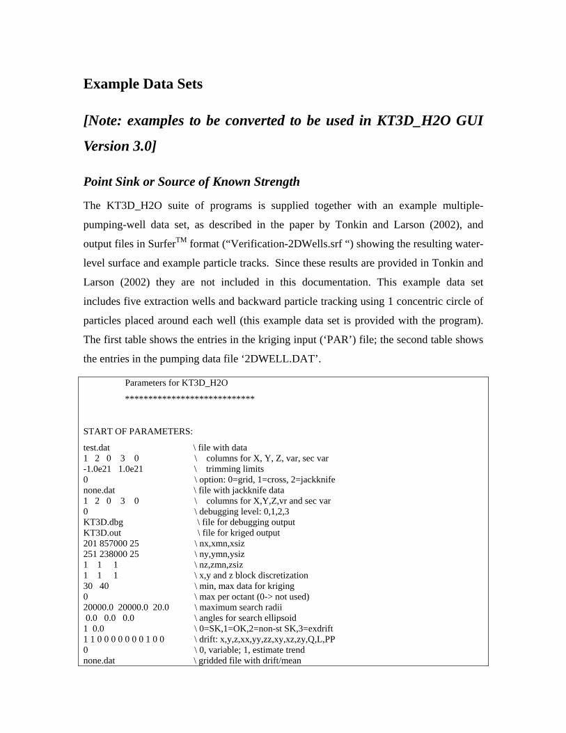
Example Data Sets
[Note: examples to be converted to be used in KT3D_H2O GUI
Version 3.0]
Point Sink or Source of Known Strength
The KT3D_H2O suite of programs is supplied together with an example multiple-
pumping-well data set, as described in the paper by Tonkin and Larson (2002), and
output files in SurferTM format (“Verification-2DWells.srf “) showing the resulting water-
level surface and example particle tracks. Since these results are provided in Tonkin and
Larson (2002) they are not included in this documentation. This example data set
includes five extraction wells and backward particle tracking using 1 concentric circle of
particles placed around each well (this example data set is provided with the program).
The first table shows the entries in the kriging input (‘PAR’) file; the second table shows
the entries in the pumping data file ‘2DWELL.DAT’.
Parameters for KT3D_H2O
****************************
START OF PARAMETERS:
test.dat \ file with data 1 2 0 3 0 \ columns for X, Y, Z, var, sec var -1.0e21 1.0e21 \ trimming limits 0 \ option: 0=grid, 1=cross, 2=jackknife none.dat \ file with jackknife data 1 2 0 3 0 \ columns for X,Y,Z,vr and sec var 0 \ debugging level: 0,1,2,3 KT3D.dbg \ file for debugging output KT3D.out \ file for kriged output 201 857000 25 \ nx,xmn,xsiz 251 238000 25 \ ny,ymn,ysiz 1 1 1 \ nz,zmn,zsiz 1 1 1 \ x,y and z block discretization 30 40 \ min, max data for kriging 0 \ max per octant (0-> not used) 20000.0 20000.0 20.0 \ maximum search radii 0.0 0.0 0.0 \ angles for search ellipsoid 1 0.0 \ 0=SK,1=OK,2=non-st SK,3=exdrift 1 1 0 0 0 0 0 0 0 1 0 0 \ drift: x,y,z,xx,yy,zz,xy,xz,zy,Q,L,PP 0 \ 0, variable; 1, estimate trend none.dat \ gridded file with drift/mean

4 \ column number in gridded file 1 0.0 \ nst, nugget effect 1 1.0 0.0 0.0 0.0 \ it,cc,ang1,ang2,ang3 20000.0 20000.0 20.0 \ a_hmax, a_hmin, a_vert 1 500 100. 0.2 1.0 8 50. 1 5 \ tracking: iback,nptp,hydcond,porosity,stepsize,nparticles,xprad,nrads,nout 1.e-4 1.e-10 0.80 1.e-6 1.e-3 \roerr,tiny,safety,eps,vsmall #note - the code knows if particle tracking has been selected by an integer flag passed #from the VB GUI to the KT3D_H2O DLL 5 858951 242823 43316 R 859806 239179 43315 R 857654 241948 52941 R 859752 241291 43316 R 860383 240985 48128 R
Horizontal Line Sink or Source of Known Strength
The KT3D_H2O suite of programs is supplied together with an example multiple-line
sink/source data set and output files in SurferTM format (“Verification-2DSink.srf “)
showing the resulting water-level surface and example particle tracks. This example data
set includes two line sinks (this example data set provided with the program). The first
Figure 5 2D Sink of Known Strength: (i) Sinks, (ii) MODFLOW, (iii) Ordinary
Kriging (no Sink Drift) (iv) 2D Sink Drift. Blue – monitoring locations.

table shows the entries in the kriging input (‘PAR’) file; the second table shows the
entries in the line segment file ‘2DSINK.DAT’. Images from the results are provided as
Figure 5. The slight discrepancy between the MODFLOW model and KT3d_H2O results
is due to the MODFLOW discretization and the proximity of the constant head boundary.
Parameters for KT3D ******************* START OF PARAMETERS: wl-2DSINK.DAT \ file with data 1 2 0 3 0 \ columns for X, Y, Z, var, sec var -1.0e21 1.0e21 \ trimming limits 0 \ option: 0=grid, 1=cross, 2=jackknife none.dat \ file with jackknife data 1 2 0 3 0 \ columns for X,Y,Z,vr and sec var 0 \ debugging level: 0,1,2,3 kt3d.dbg \ file for debugging output kt3d.out \ file for kriged output 101 6100.01 50 \ nx,xmn,xsiz 101 6100.01 50 \ ny,ymn,ysiz 1 1 1 \ nz,zmn,zsiz 1 1 1 \ x,y and z block discretization 40 40 \ min, max data for kriging 0 \ max per octant (0-> not used) 20000.0 20000.0 1.0 \ maximum search radii 0.0 0.0 0.0 \ angles for search ellipsoid 1 0.0 \ 0=SK,1=OK,2=non-st SK,3=exdrift 1 1 0 0 0 0 0 0 0 0 1 0 \ drift: x,y,z,xx,yy,zz,xy,xz,zy,Q,R,PP 1 \ 0, variable; 1, estimate trend none.dat \ gridded file with drift/mean 4 \ column number in gridded file 1 0.0 \ nst, nugget effect 1 5.0 0.0 0.0 0.0 \ it,cc,ang1,ang2,ang3 15000.0 15000.0 1.0 \ a_hmax, a_hmin, a_vert 1 100 100. 0.2 1.0 -1 50. 1 \ tracking: iback,nptp,hydcond,porosity,stepsize,nparticles,xprad,nrads 1.e-4 1.e-10 0.80 1.e-6 1.e-3 \roerr,tiny,safety,eps,vsmall #note - the code knows if particle tracking has been selected by an integer flag passed #from the VB GUI to the KT3D_H2O DLL 2 7145.00 10270.00 1 -38.6 9845.00 10270.00 1 -38.6 10420.00 7595.00 1 -75 10420.00 8295.00 1 –75

Circular Leaking Pond of Known Strength
Example data including water elevations and pond drift parameters are listed in the tables
below. Output files showing the resulting water-level surface are supplied in SurferTM
format (“CircDriftEx.srf“). Images from the results are shown here.

X Y Head Well Name7583 10691 100.887305 T18339 7422 100.774772 T210858 8022 100.981328 T39867 9993 102.713499 T411041 10067 101.36511 T57641 9718 100.935022 T67996 9174 101.00069 T78721 10879 101.181256 T89821 9777 102.583003 T912196 8674 100.851355 T109814 11990 100.989186 T1110704 8420 101.121289 T1211320 9630 101.221638 T139064 7512 100.866058 T1410962 10836 101.236196 T159411 10192 101.797811 T1611220 7977 100.91872 T1711713 10338 101.062477 T189775 8894 101.435422 T199125 10467 101.472925 T20
Data Used for Verification of KT3D_H20 Circular Pond Drift
Drift Parameters Used for Verification of KT3D_H20 Circular Pond DriftX Y Radius Strength Drift Term
10000 10000 186 0.1 1

Acknowledgements
We offer sincere gratitude to Charles Fitts, of Fitts Solutions, ME, for his invaluable
guidance when we encountered difficulties programming the line sink/source. The
correspondence that successfully led to the inclusion of this drift term helped greatly with
our understanding of the Analytic Element Method.
Technical Support
Limited technical support can be obtained by writing to [email protected].
Frequently Asked Questions
How can I make a map of my ‘best-fit’ drift (trend) surface, assuming that the errors in
the measurement data are uncorrelated, just to see a map of it?
This is analogous to performing a least-squares fit of the function:
Z = A + BX + CY + D(Q) + E(L) + F(P) + ε
… where A, B, C, D, E and F are drift coefficients; X,Y are Cartesian coordinates; Q is
the 2-D well drift component summation; L is the known strength line sink/source drift
component summation; P is the known strength circular elements drift component
summation. The error term (i.e. residual) is not included - the gridded surface will not be
an exact interpolator but will be the best fit of the trend. Theoretically, fitting of this
surface is achieved using a horizontal (‘pure nugget’) variogram. With the code provided,
this is achieved by setting the variogram parameters a_hmin, a_hmax, a_vert to 0.1, 0.1,
0.1, and setting the trend variable to 1 (‘estimate trend’).
Should I include water levels measured in extraction wells in the observed water level
data set?
Since the linear-log drift accounts for the effects of extraction or injection, water levels
measured in extraction wells should in general not be used as observations. The kriging
code as currently written does not account for linear/non-linear well losses at extraction
wells, and hence the drift coefficients (and map) will be biased by these effects, if in fact

a division-by-zero error is not encountered first (see below). There are plans to add an
additional drift term to account for linear well losses during the kriging as an additional
drift term. Please write to [email protected] if you feel this drift term would be valuable to
your needs.
The code reports a division-by-zero error upon execution.
Check that none of your extraction/injection wells and observation (monitoring) wells are
collocated – i.e. have the same X and Y coordinates. This will cause a division-by-zero
error in the estimation of the drift terms since the separation distance is zero. The current
version of the kriging program checks for co-located wells and should identify these and
terminate with an error message.
The code reports NAN (the Fortran ‘not-a-number’ flag) for an estimation point and/or
for a lagrange multiplier.
Check that none of your estimation points - i.e. a node point for which we were asking
the code to give an estimate - and observation (monitoring) wells are collocated – i.e.
have the same X and Y coordinates. This may cause an error in estimating the kriging
weights under some circumstances since the separation distance is zero. The current
version of the kriging program checks for co-located wells and should identify these and
terminate with an error message reporting the conflict(s).
NOTE: Every effort should be made to ensure there are no collocation conflicts - either
extraction wells at the same location as observation wells or observation wells at the
same location as an estimation point. This can be done in one of two ways - (1) the user
should check these conflicts will not occur; (2) by pragmatically by simply adding some
small delta-d to the observation well location coordinates. The latter, pragmatic approach
of adding some delta-d value to the X or Y of the observation points should in the
majority of instances avoid these conflicts without affecting results or their interpretation
however the magnitude of the value delta-d will be case specific.
I get a division-by-zero error, but have checked all my data and have no collocated wells
or points.

This can occur where, for example, the data set contains one extraction well, and one
injection well, and these wells form a recirculation system with extraction equaling
injection. This can be pragmatically overcome by adding a small delta-q to one of the
wells. Again, this is a pragmatic solution, and delta-q is case-specific.
Notes on an Arbitrary 2-D Polyline Boundary
A drift was incorporated in KT3D_H2O at one time to provide a general method for
representing fairly distant rivers and other extended length features. This approach is not
as rigorously founded as the drifts described in this document. The drift was derived on
the basis of an infinite, fully penetrating line sink:
• in a confined aquifer there is no curvature of the water table and the slope
towards the boundary feature is planar
• in an unconfined aquifer with no recharge the curvature of the water table
approximates a quadratic.
This form of drift term is implemented as:
Rp
ij h r a1 h +⎟
⎠⎞
⎜⎝⎛=
Where hij is the elevation of the potentiometric surface at location (i,j); a is a scalar that
is a function of T, recharge, and aquifer type; p is a power term which is typically
specified as 0.5 but is a function of the penetration of the feature; r is the distance of
location (i,j) from the boundary feature; and hR is the elevation of the boundary feature.
The user can provide an arbitrary power for the drift ranging from 1.0 (i.e., linear)
approximating the simple confined case, to 0.5 (i.e., quadratic) approximating the second
case. Note that the drift does not presently account for a slope in this feature – e.g., a bed
slope in a river across the data domain. NOTE: In the current version of KT3D_H2O this
drift term is disabled. Please contact [email protected] if this drift may suite your needs.

References
Brochu, Y. and Marcotte, D., (2003). A simple approach to account for radial flow and
boundary conditions when kriging hydraulic head fields for confined aquifers.
Mathematical Geology, Vol. 35, No. 2, February 2003.
Chiles, J., and P. Delfiner. 1999. Geostatistics: Modeling Spatial Uncertainty. New York:
John Wiley & Sons.
Deutsch, C., and Journel, A., (1992). GSLIB: Geostatistical Software Library and User's
Guide. Oxford University Press, 340 pp.
Ferris, J.G., D.B. Knowles, R.H. Brown, and R.W. Stallman (1962). Theory of aquifer
tests. U.S. Geological Survey Water-Supply Paper 1536-E.
Fitts, C., (2004). TWODAN - Manual. Fitts Geosolutions, Scarborough, Maine.
McDonald, M.G., and Harbaugh, A.W., (1988). A modular three-dimensional finite-
difference ground-water flow model. U.S. Geological Survey Techniques of
Water-Resources Investigations, book 6, chap. A1, 586 p.
Pollock, D.W., (1994). User's Guide for MODPATH/MODPATH-PLOT, Version 3: A
particle tracking post-processing package for MODFLOW, the U.S. Geological
Survey finite-difference ground-water flow model. U.S. Geological Survey Open-
File Report 94-464, 234 p.
Press, W. H., B. P. Flannery, S. A. Teukolsky and W. T. Vetterling, (1996), Numerical
Recipes in Fortran-90. Vol. 2. 2nd edn., Cambridge University Press, Cambridge.
Reilly, T.E., O.L. Franke and G.D. Bennett, (1987). The principal of superposition and its
application in ground-water hydraulics. USGS Techniques of Water Resources
Investigations of the United States Geological Survey, Book 3, Chapter B6.
Strack, O.D.L., (1989). Groundwater Mechanics. Prentice-Hall, Englewood Cliffs, New
Jersey.
Tonkin, M.J., and Larson, S.P., (2002). Kriging water levels with a regional-linear and
point-logarithmic drift. Ground Water, 40 (2), 185-193, March/April.
Volpi, G., and Gambolati, G., (1978). On the use of a main trend for the kriging
technique in hydrology. Advances in Water Resources, 1, 345-349.

Zheng, C., (1992). PATH3D: A Groundwater Path and Travel-Time Simulator, Version
3.0, S.S. Papadopulos & Associates, Inc., Bethesda, Maryland.

Appendix A: Kriging Water Levels with a Regional-linear and
Point-logarithmic Drift, Ground Water, 2002
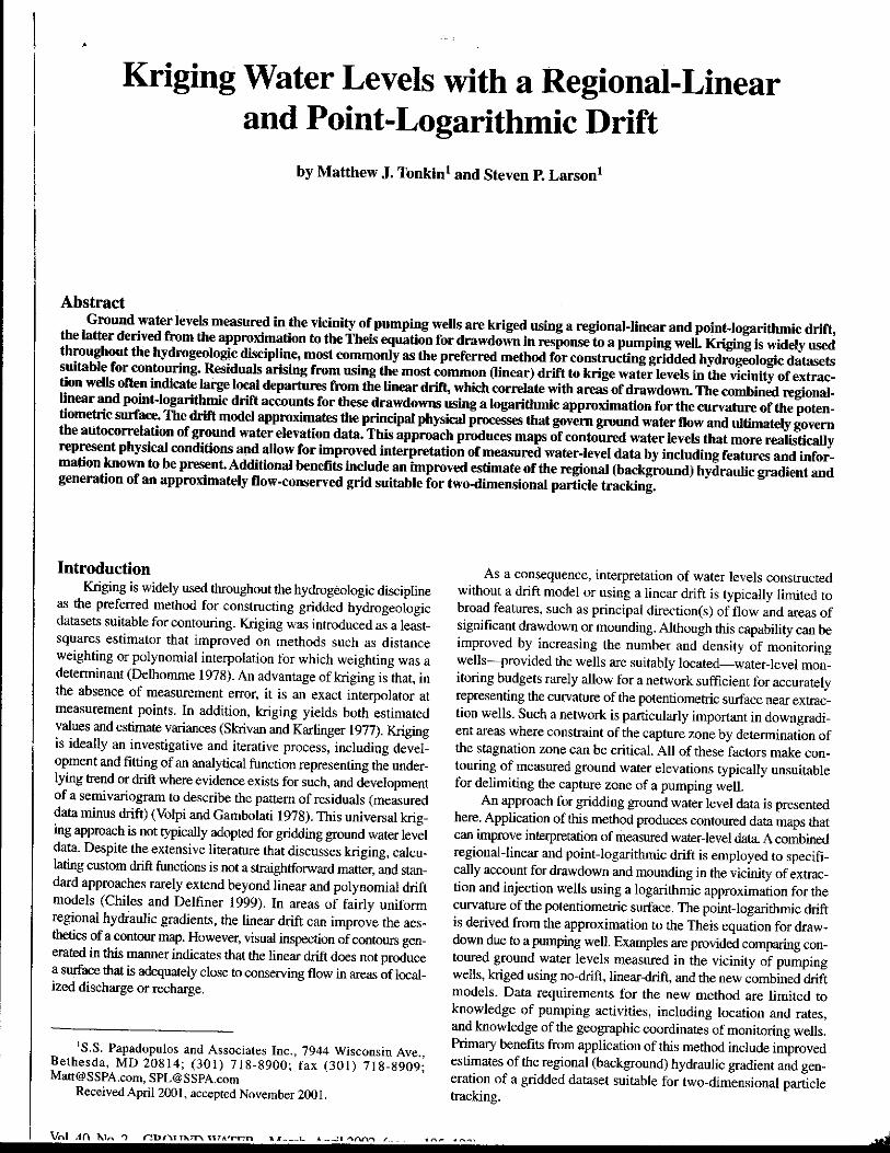
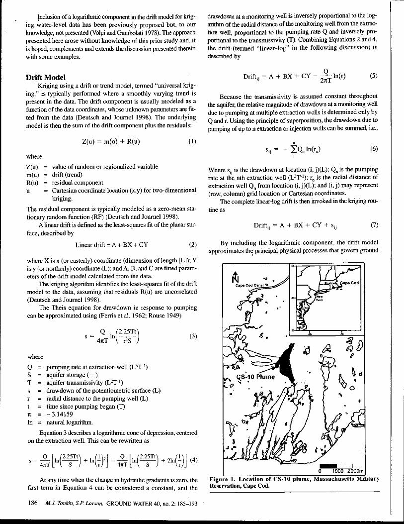


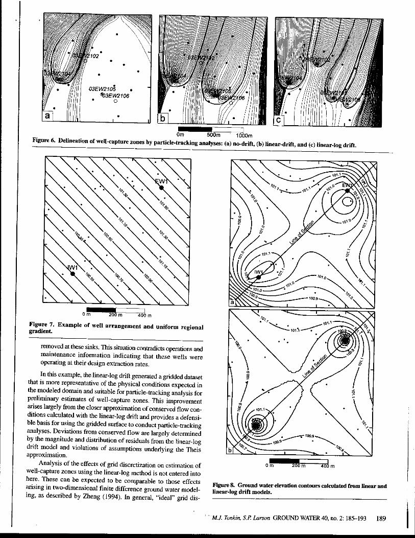


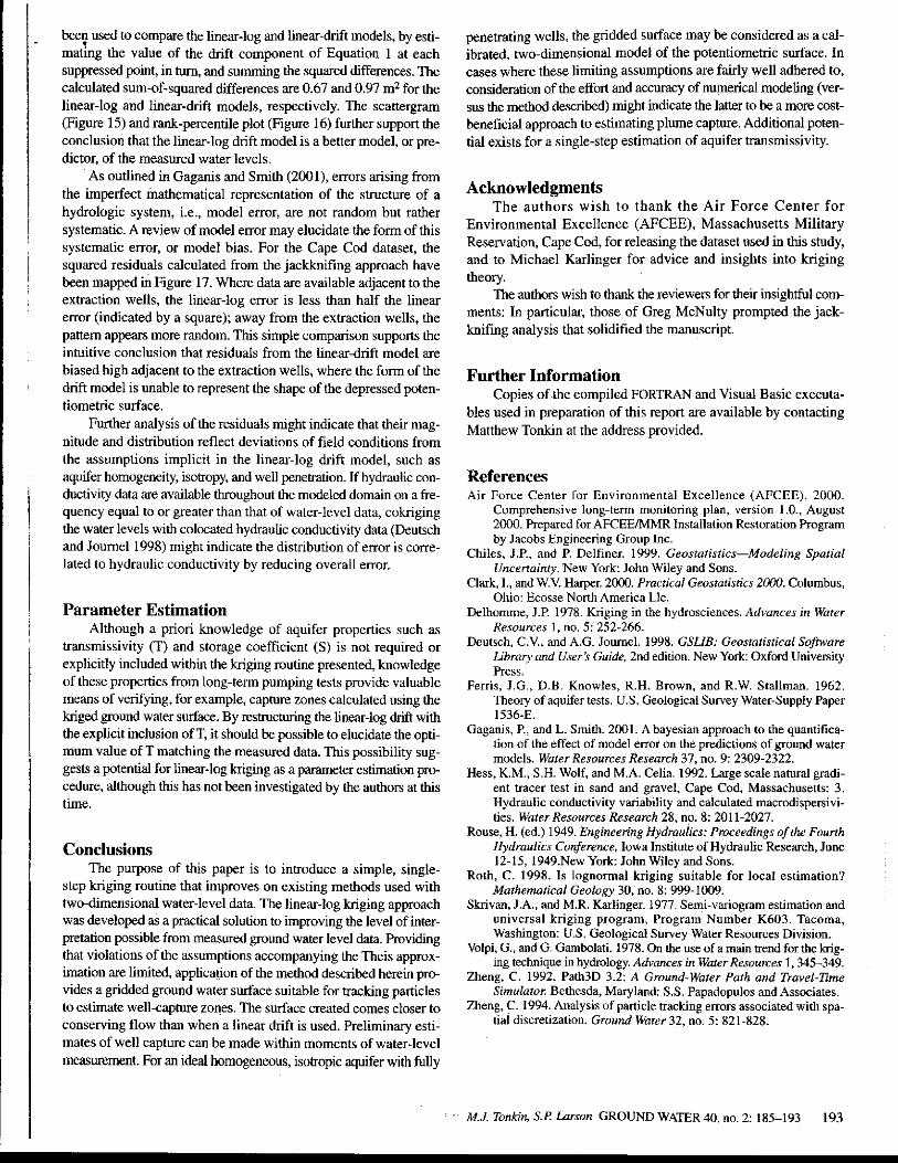

Attachment 2 Documentation and Verification Package for TransientTracker
Documentation and Veri�cation Package for:
TransientTracker
A Program for Conducting Particle Tracking
i
Contents
Contents i
List of Figures ii
Outline iii
1 TransientTracker 1
1.1 Background . . . . . . . . . . . . . . . . . . . . . . . . . . . . . . . . 1
1.2 Approach . . . . . . . . . . . . . . . . . . . . . . . . . . . . . . . . . 1
1.3 Principal Program Routines . . . . . . . . . . . . . . . . . . . . . . . 2
1.4 Input . . . . . . . . . . . . . . . . . . . . . . . . . . . . . . . . . . . . 2
1.5 Output . . . . . . . . . . . . . . . . . . . . . . . . . . . . . . . . . . . 8
2 Program Veri�cation Data Set 9
2.1 Veri�cation with Travel Time Derived From Thiem Equation . . . . 10
2.2 Veri�cation with Analytical Solution, BRICK . . . . . . . . . . . . . 10
2.3 Veri�cation Using Numerical Solutions . . . . . . . . . . . . . . . . . 12
References 20
A Surfer ASCII Grid File Format 21

ii
List of Figures
1 Example head surface near a pumping well (red circle) calculated using
a) bilinear interpolation and b) linear-log kriging. . . . . . . . . . . . 3
2 Example particle tracks using the linear-log kriging approach. . . . . 4
3 Travel time to reach pumping well calculated using (1) analytical so-
lution, (2) MODPATH, and (3) TransientTracker. . . . . . . . . . . . 11
4 Particles from TransientTracker and contours from BRICK at T =
1000days. . . . . . . . . . . . . . . . . . . . . . . . . . . . . . . . . . 12
5 Particles from TransientTracker for 2 dispersivity values and zero dis-
persivity at T=1000days. . . . . . . . . . . . . . . . . . . . . . . . . . 13
6 Test case model grid with GHB cells (blue) and pumping cell (red).
Each grid cell is 100 feet on each side. The grid has 100 columns and
50 rows. . . . . . . . . . . . . . . . . . . . . . . . . . . . . . . . . . . 13
7 Initial groundwater surface. . . . . . . . . . . . . . . . . . . . . . . . 15
8 Final groundwater surface. . . . . . . . . . . . . . . . . . . . . . . . . 15
9 Comparison of TransientTracker and MODPATH results, no dispersion. 16
10 TransientTracker particle paths with longitudinal (2.5 feet) and trans-
verse (0.5 feet) dispersion. . . . . . . . . . . . . . . . . . . . . . . . . 17
11 Particle locations (black) at 8688.7 days. . . . . . . . . . . . . . . . . 17
12 Dispersion impacted TransientTracker particles from a point source at
8688.7 days, with the advection-only track in the packground. . . . . 18
13 Capture zone indicating the locations (black circles) from which a parti-
cle released will be captured by the recovery well. Gray crosses indicate
particles that leave through a domain boundary. . . . . . . . . . . . . 18
14 Order data must be written for Surfer grid �le. . . . . . . . . . . . . . 21

iii
Outline
This document describes a program, TransientTracker, for calculating approximate
travel paths. TransientTracker requires as input at least one grid of hydraulic head.
This grid can be generated by any number of methods including: interpolation of
observations, analytical solutions, and numerical simulation results.
Use of the program should be accompanied by review of the references and dis-
claimer provided at the end of this Documentation and Veri�cation Package.
TransientTracker is programmed in Fortran 90/95 using a modular program struc-
ture. TransientTracker has been developed to be independent of any speci�c model
platform, requiring simple ASCII input �les and producing ASCII output �les. The
programs can be obtained free of charge, together with an example data set, by writ-
ing to [email protected]. The performance of TransientTracker has been tested in a
variety of applications. Future applications, however, might reveal errors that were
not detected in the test simulations. Users are requested to notify [email protected] of
any errors found in this document or the programs.

1
1 TransientTracker
1.1 Background
Particle tracking has been implemented in TransientTracker to support approximate
evaluations of historic and future contaminant migration; of hydraulic capture zones
developed by pump-and-treat type remedies; and other analyses that bene�t from the
ability to track particles on a surface. Inputs required to execute particle tracking
using TransientTracker are described in the following section. The particle track-
ing implemented in TransientTracker is currently only compatible with 2-D surfaces,
which must be provided to TransientTracker as a formatted input.
Particle tracking uncertainty, associated with the physical process of hydrody-
namic dispersion and mixing, is incorporated through a random walk component.
The random walk movements are added to the advective displacements, providing an
indication of the expected uncertainty in particle location due to dispersion. Larger
numbers of particles will provide a better representation of the potential for plume
spreading due to dispersion, but will add signi�cantly to computation time.
1.2 Approach
Particle tracking is implemented using the fourth-order Runge-Kutta (RK4: Press
et al. 1992) numerical integration (particle tracking) scheme, calculated upon hy-
draulic head surfaces that have been generated using any number of methods including
analytical solutions, interpolation of observed values or a numerical simulation such
as MODFLOW (McDonald and Harbaugh 1988). This particle tracking approach can
be used to indicate the (relative) timing of the arrival of contaminants at potential re-
ceptors and/or points of calculation (POCs). This particle tracking approach is based
upon that implemented in the MODFLOW-compatible particle-tracking code Path3D
(Zheng 1992), which has been demonstrated to provide very similar results to the
USGS particle tracking program MODPATH (Pollock 1994). The RK4 scheme that
is being employed also incorporates Random-Walk (RW) approaches for representing
the spreading of contaminants through time due to dispersive e�ects (Prickett et al.
1981; Zheng and Bennett 2002). Either of the approaches, Prickett et al. (1981) or
Zheng and Bennett (2002), are available, selected by a �ag in the input �le (see input
instructions below). It is noted that these methods are not mass conservative � that
is, while they can consider the a�ects of advection, retardation and dispersion, they
do not consider or conserve the mass of contaminants that are in the groundwater.
The method employed by TransientTracker o�ers a rapid, visual means, of assessing

2
the potential uncertainties in solute transport directions, which will be critical for
e�cient evaluation of large numbers of potential scenarios and assessing impacts of
parameter uncertainty.
TransientTracker uses the linear-log kriging (pumping well drift) approach of
Tonkin and Larson (2002) to calculate a more reasonable representation of the veloc-
ity �eld near pumping wells compared with a bilinear interpolation scheme (Figure 1.
In addition, the velocity �eld converges on the well (Figure 2), which can be expected
to produce more reasonable capture zones.
1.3 Principal Program Routines
The principal routines in the code are listed below, along with brief descriptions.
rkasc: (and rk4) These two routines perform a 4th Runge-Kutta solution to de-
termine the future particle location. The routine rkasc monitors trunca-
tion error and performs step-size adjustment, while rk4 handles the mul-
tiple calls to the velocity-interpolation routine, accumulates the multiple
estimates and weights them to provide the updated particle location.
vpoint: This routine performs simple linear interpolation of velocity between grid-
nodes. The routine also checks for strong sinks, or strong sinks in adjacent
cells. When evaluating velocity in weak-sink cells the routine invokes an
analytical solution to determine the velocity vector within a cell.
krig: Kriging algorithm from Skrivan and Karlinger (1977) used to calculate
velocities for particles near wells according to the method described by
Tonkin and Larson (2002).
pzdispersion: Particle dispersion is implemented through this routine using either
Prickett et al. (1981) or Zheng and Bennett (2002) depending on the �ag
setting in the input �le. This routine is not invoked if all dispersivities
are set to 0.0 in the input �le.
1.4 Input
TransientTracker reads up to four types of input �les. The �rst one is the main input
�le, TransientTracker.in, and is required and must have the default name. The other
three types are Surfer grid �les (GRDFILES), Well �les (WELFILES), and Sink �les
(LINEFILES). All of these �les are listed by name in TransientTracker.in.

3
(a) Bilinear interpolation
(b) Linear-log Kriging
Figure 1: Example head surface near a pumping well (red circle) calculated using a)bilinear interpolation and b) linear-log kriging.

4
Figure 2: Example particle tracks using the linear-log kriging approach.
The following table provides a summary of the variables required in the default in-
put �le, TransientTracker.in, in the format required by the code. The indices indicate
the order in which the variables are listed in the �le, a new line for each successive
index, with some variables requiring multiple lines of input. Text in lowercase-bold
are character variables: they need to be entered exactly as provided in the table,
followed by the variables indicated. The input is free format: entries do not need a
speci�c spacing on each line, and multiple entries on a line should be separated by
one or more spaces.
Index Variables
1 ngrd NGRD2 ncol NCOL3 nrow NROW4 xmn XMN5 ymn YMN6 zmn ZMN7 GRDFILES(i), WELFILES(i), LINEFILES(i), TTIME(i): This line is
repeated NGRD times8 IBACK, NPTP, COND, POR, STEP, NPART, XPRAD, NRADS,
NOUT, MAXTIME9 ALPL, ALPT, PORZ
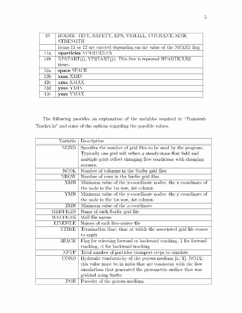
5
10 ROERR, TINY, SAFETY, EPS, VSMALL, COURANT, SINKSTRENGTHItems 11 or 12 are entered depending on the value of the NPART �ag
11a nparticles NPARTICLES11b XPSTART(j), YPSTART(j): This line is repeated NPARTICLES
times.12a space SPACE12b xmn XMIN12c xmx XMAX12d ymn YMIN12e ymx YMAX
The following provides an explanation of the variables required in �Transient-
Tracker.in� and some of the options regarding the possible values.
Variable Description
NGRD Speci�es the number of grid �les to be used by the program.Typically one grid will re�ect a steady-state �ow �eld andmultiple grids re�ect changing �ow conditions with changingstresses.
NCOL Number of columns in the Surfer grid �lesNROW Number of rows in the Surfer grid �lesXMN Minimum value of the x-coordinate nodes: the x coordinate of
the node in the 1st row, 1st columnYMN Minimum value of the y-coordinate nodes: the y coordinate of
the node in the 1st row, 1st column.ZMN Minimum value of the z-coordinate
GRDFILES Name of each Surfer grid �leWELFILES Well �le namesLINEFILE Names of each line-source �le
TTIME Termination time, time at which the associated grid �le ceasesto apply
IBACK Flag for selecting forward or backward tracking. 1 for forwardtracking, -1 for backward tracking
NPTP Total number of particles transport steps to simulateCOND Hydraulic conductivity of the porous medium [L/T]. NOTE:
this value must be in units that are consistent with the �owsimulations that generated the piezometric surface that wasgridded using Surfer
POR Porosity of the porous medium

6
STEP Transport step size for moving particlesNPARTXPRAD Placeholder value for future useNOUT Transport step interval for output, e.g., NOUT = 5 will
produce output every 5th transport stepMAXTIME Maximum simulation time
ALPL Longitudinal dispersivity [L]. NOTE: this value must be inunits that are consistent with the �ow simulations thatgenerated the piezometric surface that was gridded using Surfer
ALPT Transverse dispersivity [L]. NOTE: this value must be in unitsthat are consistent with the �ow simulations that generatedthe piezometric surface that was gridded using Surfer
PORZ Flag to indicate which formulation of the random-walkdispersion approximation is used: PORZ = 0 for Prickett et al.(1981), or PORZ = 1 for Zheng and Bennett (2002)
ROERR Round-o� error cuto� for Runge-Kutta integration(recommended = 1.0 E-04)
TINY Stagnation and minimum tracking time criterion forRunge-Kutta integration (recommended = 1.0 E-10)
SAFETY Stepsize adjustment criterion for Runge-Kutta integration(recommended = 0.80)
EPS Error criterion scaling factor for Runge-Kutta integration(recommended = 1.0 E-06)
VSMALL Placeholder value for future use. (recommended =SQRT(EPS))
COURANT Particle step control. If the updated particle location moves aparticle more than 1 cell length, the step size is recalculatedusing the courant number according to: courant×cell size
magnitude of velocity
SINKSTRENGTH Used to �ag low-points in the �ow �eld that are not the resultof a well or line-sink. These low-points are stagnation areas forparticles and cause lengthy runtimes if a particle is allowed to�bounce� around in these areas. The strength is a headdi�erence. That is, if the head at a node is more thanSINKSTRENGTH less than the value of the four surroundingnodes, that node is �agged as an internal sink
NPARTICLES Number of particles to simulate if NPART is 1XPSTART Starting x-coordinate location for particleYPSTART Starting y-coordinate location for particle
SPACE If NPART is 0 then a regular grid of particles is simulated.SPACE is the spacing between particles for this grid
XMIN minimum x-coordinate for particle location gridXMAX maximum x-coordinate for particle location gridYMIN minimum y-coordinate for particle location grid

7
YMAX maximum y-coordinate for particle location grid
GRDFILES(i) The Surfer input �les, the GRDFILES(i), listed in TransientTracker.in,
are grids of the groundwater levels from each timestep of the numerical
simulation. The grids are associated with the total elapsed simulation
time (TTIME(i)) at the end of each respective timestep. To avoid poten-
tial issues with location referencing, all grids must have the same dimen-
sions and origins. Formatting instructions for creating Surfer ASCII �les
is includedin Appendix A of this manual.
WELFILES(i): The �les de�ning the locations and characteristics of each well are
simple ASCII �les and provide information in the following format:
Index Variable
1 NWELLS2 qxx(i),qyy(i),qqq(i),qrad(i),idtwell(i),qtype(i),wellname(i) where this
line is repeated NWELLS times.
The parameters listed above have the following de�nitions:
Variable Description
NWELLS Speci�es the number of wells �les that are active during thistimestep: the wells that in�uenced the current grid �le.
qxx(i) X �coordinate of well iqyy(i) Y �coordinate of well iqqq(i) Pumping rate of well i for the current timestepqrad(i) Well bore radius. Used to capture the particles as they
approach the well. In some instances, especially with wellscreating a very sharp cone of depression, increasing thisnumber beyond the actual well-bore radius may help withstability of the �nal particle transport steps.
idtwell(i) A well-id labelqtype(i) Specify the well as recovery (R) or not recovery (NR)
wellname(i) A name for the well
LINEFILES(i): These �les de�ne the locations and characteristics of sink line seg-
ments. They are simple ASCII �les and provide information in the fol-
lowing format:

8
Index Variable
1 NLIN2 lxs(i),lys(i),lind(i),lval(i) where this line is repeated NLIN times.3 lxe(i),lye(i),idum,rdum
NOTE: Items 2 and 3 are repeated NLIN times. If NLIN <0 then only2 is repeated NLIN times.
The parameters listed above have the following de�nitions:
Variable Description
NLIN Number of line segments to be read in the �le. Must be lessthan 100, which is hardwired into the code as MAXNLIN
lxs(i) X location of starting point(s) ilys(i) Y location of starting point(s) ilind(i) Indicator of line sink/source/'feature' type. 1 - 'river' with a
const head value, 2 - 'horiz well' with const Q-in/Q-outLval(i) 'value' for the line feature. Head (when lind = 1), river (when
lind = 1)lxe(i) X location of ending point(s)lye(i) Y location of ending point(s)
idum(i) Check value, needs to match lvalrdum(i) Check value, needs to match lind
1.5 Output
TransientTracker produces two output �les: the particle tracks, ptrack.out, and the
capture locations of each particle, capture.out. Both ptrack.out and capture.out are
formatted ASCII �les that can easily be imported by a plotting package such as
Surfer.
The �le ptrack.out provides a listing of the particle locations (x, y, time, particle
number) with each transport step (or multiple of transport steps depending on the
value of NOUT). A sample of the �rst few lines of a typical ptrack.out �le is provided
below:
0.374760000000E+04 0.413894000000E+04 0.000000000000E+00 1
0.374879680903E+04 0.413927856838E+04 0.200000000000E+00 1
0.374733118239E+04 0.413823623645E+04 0.100000000000E+01 1
TransientTracker includes functionality for removing particles at the margins of
the grid domain; at stagnation zones; at sinks when forward tracking. The program
records the fate of particles in an ASCII summary �le called capture.out. The contents
of this �le can be manipulated to illustrate capture zones. The program uses an integer

9
variable (IREM) to indicate if, and where, a particle was removed from the particle
tracking for any of the reasons listed above. The value of this variable, as written
to capture.out can be used to produce maps that illustrate the fate of the particles.
Current capabilities include the removal of particles that exit the domain:
• Not captured (IREM=0)
• At the bounds of the grid (IREM=1)
• At a 2D Recovery Well (IREM=2) (QTYPE='R')
• At a 2D line sink/sources (IREM=3)
• At a stagnation point (IREM=5 or 6)
• Beyond the maximum transport-simulation time (IREM=8)
• Number of tracking steps exceeded (IREM=9)
• Internal stagnation point (IREM=10)
Non-recovery wells are typically injection wells, but may also be wells that are not
pumping in a particular stress period, but were simply left in the input �le for con-
sistency. The �le capture.out provides, for each particle, the starting location, exit
time, exit coordinates, exit row, column and layer, and the mechanism of exit. An
example of a portion of a capture.out �le is provided below:
1 6161.9587 1761.6945 0.0000 14852.2305 3556.8680 947.477
2 5948.3987 1685.1856 0.0000 13742.2650 3557.3389 944.395
3 5626.3664 1414.9735 0.0000 11981.5765 3553.3730 953.438
4 5870.5205 1624.0371 0.0000 13106.5835 3550.3535 943.901
2 Program Veri�cation Data Set
TransientTracker was veri�ed using two analytical solutions and a set of numerical
solutions of a two-dimensional transient system.

10
2.1 Veri�cation with Travel Time Derived From Thiem Equa-
tion
The explicit solution of the Thiem equation for particle travel time to a well (Neville
2007) was used to estimate particle travel time from a variety of distances to a fully-
penetrating well in a con�ned, homogeneous system. Results were also generated us-
ing MODFLOW and MODPATH. A Surfer grid �le was made from the MODFLOW-
calculated potentiometric surface. Particle tracking using TransientTracker and the
Surfer grid �le was performed to create a third set of results. All three sets of results
are included in Figure 3.
The results shown in Figure 3 demonstrate excellent agreement between the three
methods. The parameters used for this simulation are listed in the table below.
Parameter Value
Hydraulic Conductivity (m/day) 0.864Aquifer Thickness (m) 10.0Well radius (m) 0.1Maximum travel distance (m) 100.0Pumping rate (m3/day) 54.5Porosity 0.35MODFLOW Square grid-cell size (m) 2.0MODFLOW Grid dimensions 1001 x 1001
2.2 Veri�cation with Analytical Solution, BRICK
TransientTracker, particularly the dispersion process component, was veri�ed by com-
paring the results with an analytical solution of a simple transport scenario. The an-
alytical code BRICK (Neville 2006) was used to generate contours of concentration
at 1000 days after an initial released from a square source zone measuring 5 feet on
each side. The following inputs were speci�ed for BRICK:
Porosity [-] 0.30Velocity [L/T] 0.25Longitudinal Dispersivity [L] 10.0Lateral Transverse Dipsersivity [L] 0.1Source zone Xmin, Xmax -5.0, 5.0Source zone Ymin, Ymax -5.0, 5.0Initial Slug Mass 1.00 E+05Domain Xmin, Xmax, dx -50.0, 500.0, 1.0Domain Ymin, Ymax, dy -100.0, 100.0, 1.0

11
Figure 3: Travel time to reach pumping well calculated using (1) analytical solution,(2) MODPATH, and (3) TransientTracker.
Using an assumed value of hydraulic conductivity equal to 100.0, a Surfer grid �le
was created with the same domain extent and grid resolution as the BRICK solution.
The piezometric surface generated using a gradient of 7.5 E-04, with the high values
of piezometric surface along the left hand boundary (X = -50.0).
TransientTracker was run with the resulting Surfer Grid �le using 1681 particles
(a square of 41 x 41 particles) and dispersivity values matching the BRICK values.
The �le TransientTracker.in is provided below.
# Input file for TransientTracker benchtesting against BRICK
ngrd 1
ncol 551
nrow 201
xmn -50.00
ymn -100.00
zmn 0.
# Grid File information using 1 line for each "stress period"
fabgrid551x201.grd nowells.dat nosinks.dat 1000.
# Tracking information
1 100000 100.0 0.3 10.0 1 50. 1 1 30000.
10.0 0.1 0
1.e-3 1.e-6 0.8 1.e-6 1.0e-3 1.0 0.
# Particle Locations 1681
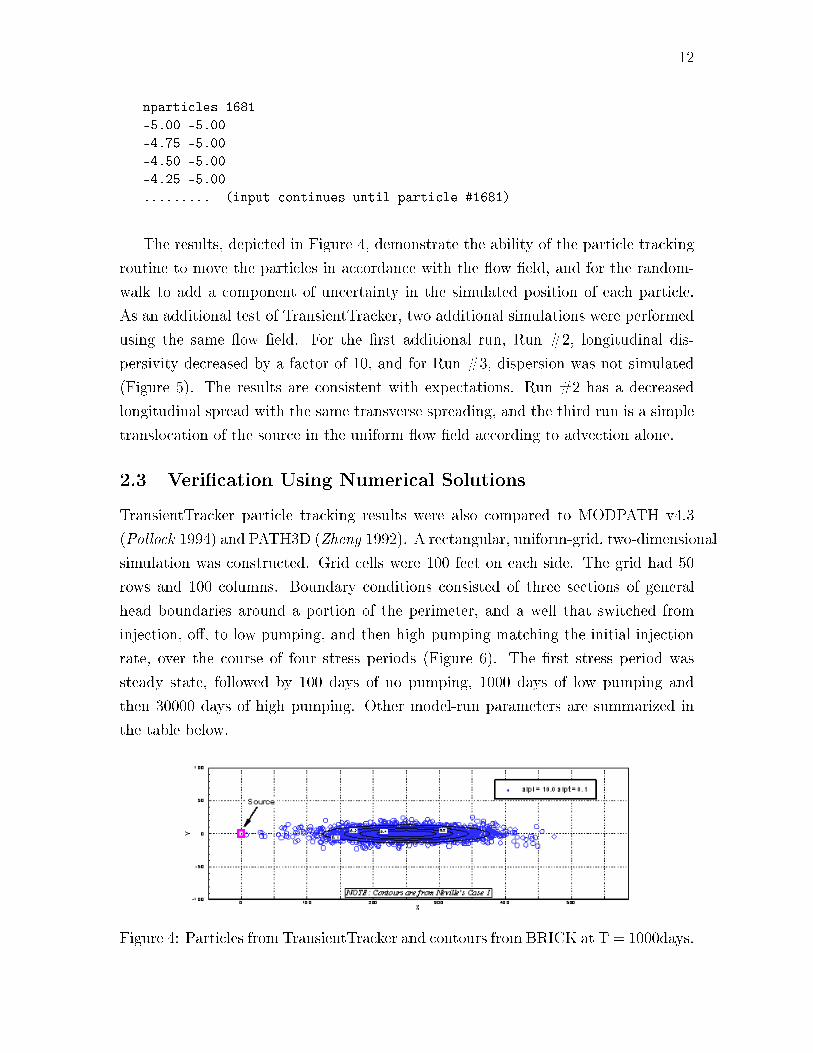
12
nparticles 1681
-5.00 -5.00
-4.75 -5.00
-4.50 -5.00
-4.25 -5.00
......... (input continues until particle #1681)
The results, depicted in Figure 4, demonstrate the ability of the particle tracking
routine to move the particles in accordance with the �ow �eld, and for the random-
walk to add a component of uncertainty in the simulated position of each particle.
As an additional test of TransientTracker, two additional simulations were performed
using the same �ow �eld. For the �rst additional run, Run #2, longitudinal dis-
persivity decreased by a factor of 10, and for Run #3, dispersion was not simulated
(Figure 5). The results are consistent with expectations. Run #2 has a decreased
longitudinal spread with the same transverse spreading, and the third run is a simple
translocation of the source in the uniform �ow �eld according to advection alone.
2.3 Veri�cation Using Numerical Solutions
TransientTracker particle tracking results were also compared to MODPATH v4.3
(Pollock 1994) and PATH3D (Zheng 1992). A rectangular, uniform-grid, two-dimensional
simulation was constructed. Grid cells were 100 feet on each side. The grid had 50
rows and 100 columns. Boundary conditions consisted of three sections of general
head boundaries around a portion of the perimeter, and a well that switched from
injection, o�, to low pumping, and then high pumping matching the initial injection
rate, over the course of four stress periods (Figure 6). The �rst stress period was
steady state, followed by 100 days of no pumping, 1000 days of low pumping and
then 30000 days of high pumping. Other model-run parameters are summarized in
the table below.
Figure 4: Particles from TransientTracker and contours from BRICK at T = 1000days.

13
Figure 5: Particles from TransientTracker for 2 dispersivity values and zero disper-sivity at T=1000days.
Figure 6: Test case model grid with GHB cells (blue) and pumping cell (red). Eachgrid cell is 100 feet on each side. The grid has 100 columns and 50 rows.
Parameter Value
Porosity [-] 0.10Longitudinal Dispersivity [ft] 2.5 or 0.0Lateral Transverse Dipsersivity [ft] 0.5 or 0.0Hydraulic Conductivity [ft/day] 100.0Stress-period Pumping [1000 ft3/day] 50, 0, -2, -50
The following sets of �gures depict results from the groundwater simulation and
the particle tracking. It is worth noting that this test case is not intended to be strictly
realistic: it was constructed to provide a set of groundwater surface elevations with
dramatic changes in the velocity vectors over time.
Figure 7 depicts the initial steady-state groundwater surface due to the general
head boundaries and the well injecting at ∼250 gpm. The particle release locations
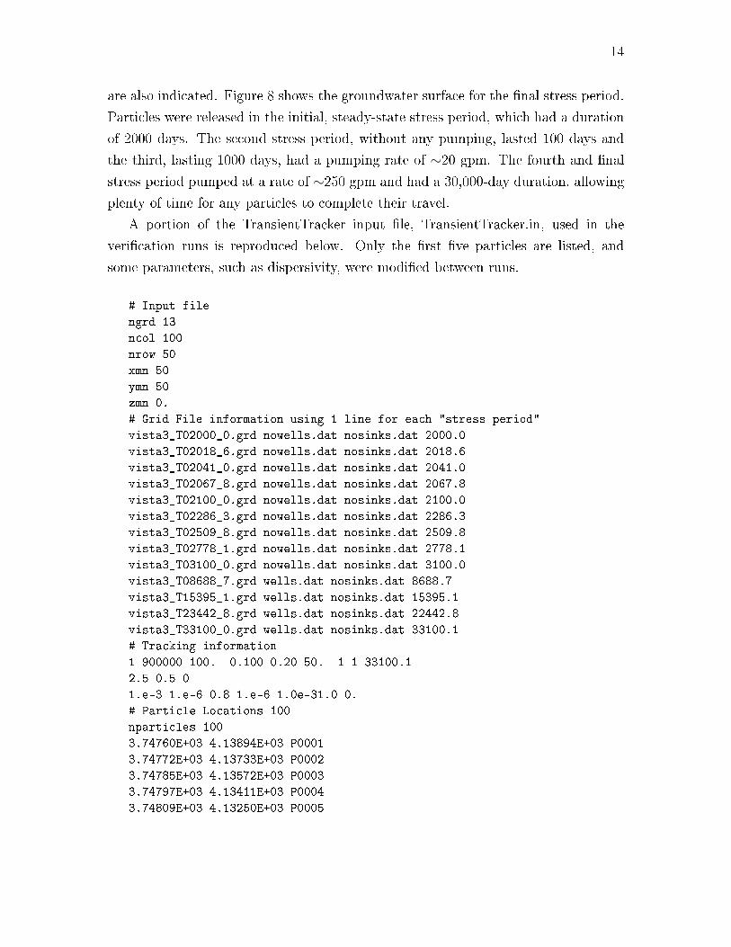
14
are also indicated. Figure 8 shows the groundwater surface for the �nal stress period.
Particles were released in the initial, steady-state stress period, which had a duration
of 2000 days. The second stress period, without any pumping, lasted 100 days and
the third, lasting 1000 days, had a pumping rate of ∼20 gpm. The fourth and �nal
stress period pumped at a rate of ∼250 gpm and had a 30,000-day duration, allowing
plenty of time for any particles to complete their travel.
A portion of the TransientTracker input �le, TransientTracker.in, used in the
veri�cation runs is reproduced below. Only the �rst �ve particles are listed, and
some parameters, such as dispersivity, were modi�ed between runs.
# Input file
ngrd 13
ncol 100
nrow 50
xmn 50
ymn 50
zmn 0.
# Grid File information using 1 line for each "stress period"
vista3_T02000_0.grd nowells.dat nosinks.dat 2000.0
vista3_T02018_6.grd nowells.dat nosinks.dat 2018.6
vista3_T02041_0.grd nowells.dat nosinks.dat 2041.0
vista3_T02067_8.grd nowells.dat nosinks.dat 2067.8
vista3_T02100_0.grd nowells.dat nosinks.dat 2100.0
vista3_T02286_3.grd nowells.dat nosinks.dat 2286.3
vista3_T02509_8.grd nowells.dat nosinks.dat 2509.8
vista3_T02778_1.grd nowells.dat nosinks.dat 2778.1
vista3_T03100_0.grd nowells.dat nosinks.dat 3100.0
vista3_T08688_7.grd wells.dat nosinks.dat 8688.7
vista3_T15395_1.grd wells.dat nosinks.dat 15395.1
vista3_T23442_8.grd wells.dat nosinks.dat 22442.8
vista3_T33100_0.grd wells.dat nosinks.dat 33100.1
# Tracking information
1 900000 100. 0.100 0.20 50. 1 1 33100.1
2.5 0.5 0
1.e-3 1.e-6 0.8 1.e-6 1.0e-31.0 0.
# Particle Locations 100
nparticles 100
3.74760E+03 4.13894E+03 P0001
3.74772E+03 4.13733E+03 P0002
3.74785E+03 4.13572E+03 P0003
3.74797E+03 4.13411E+03 P0004
3.74809E+03 4.13250E+03 P0005

15
Figure 7: Initial groundwater surface.
Figure 8: Final groundwater surface.

16
Figure 9: Comparison of TransientTracker and MODPATH results, no dispersion.
The gray particles in Figure 9 are the MODPATH particle-tracking results. The
black particles are the TransientTracker results. The two methods provide nearly
identical paths. Path3D results are not shown since they were indistinguishable from
these results. This �gure provides a demonstration that TransientTracker is capable
of representing advective particle transport in homogeneous aquifers.
Particle tracks in Figure 10 demonstrate the longitudinal (2.5 feet) and transverse
(0.5 feet) dispersivity impacts using the same line source and conditions as in Figure
9. Dispersion in this �gure is simulated using the Prickett et al. (1981) random
walk algorithm. In Figure 11 the same particle tracks are shown in the background,
and in the foreground are particle locations at 8688.7 days after the start of the
simulation. This cloud of particles illustrates the considerable di�erences in travel
time experienced by the various particles as a result of small di�erences in starting
location, and the simulated dispersion.
By starting all 100 particles at a single point, Figure 12 provides a comparison
to Figure 11 and demonstrates that the simulated dispersion, as opposed to initial
particle location, is the dominant source of spreading as the particles progress towards
the well. The advection-only particle track originating from the single-point source
is provided in the background (gray) for reference.
For remediation purposes, it is often helpful to assess the capture region for a given
scenario. The capture.out �le was used to identify locations where particles released
at the beginning of the simulation would get captured by the well. The red dots in
Figure 13 indicate the locations that will be captured by the well, while the blue
crosses indicate locations where particles move out of the domain instead of being
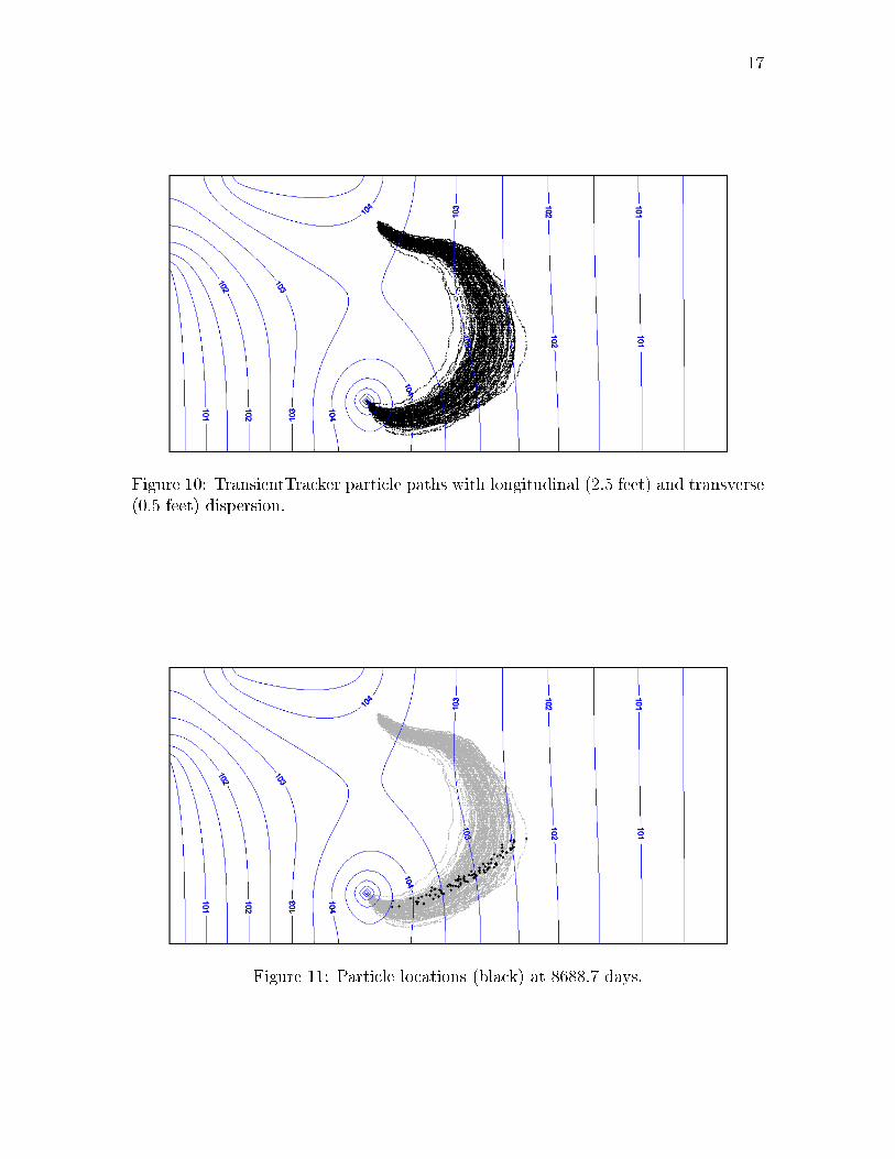
17
Figure 10: TransientTracker particle paths with longitudinal (2.5 feet) and transverse(0.5 feet) dispersion.
Figure 11: Particle locations (black) at 8688.7 days.
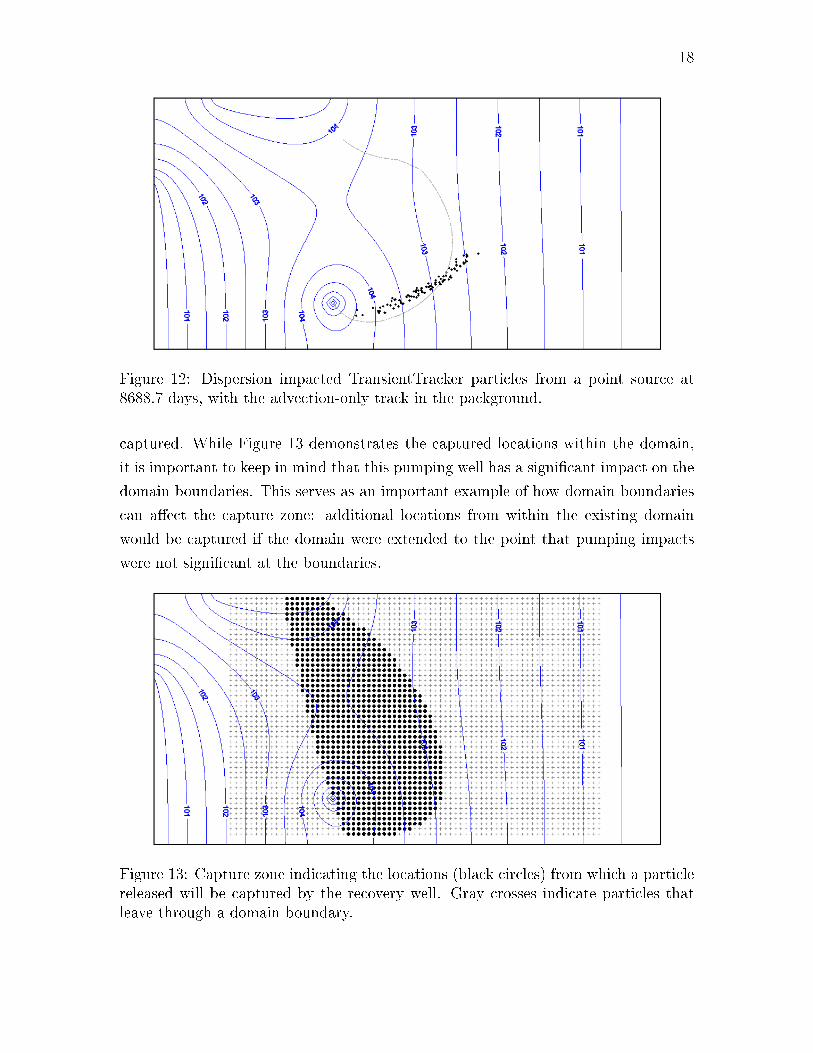
18
Figure 12: Dispersion impacted TransientTracker particles from a point source at8688.7 days, with the advection-only track in the packground.
captured. While Figure 13 demonstrates the captured locations within the domain,
it is important to keep in mind that this pumping well has a signi�cant impact on the
domain boundaries. This serves as an important example of how domain boundaries
can a�ect the capture zone: additional locations from within the existing domain
would be captured if the domain were extended to the point that pumping impacts
were not signi�cant at the boundaries.
Figure 13: Capture zone indicating the locations (black circles) from which a particlereleased will be captured by the recovery well. Gray crosses indicate particles thatleave through a domain boundary.

19
Technical Support
Limited technical support can be obtained by writing to [email protected].
Disclaimer
This software is provided "AS IS", without warranty of any kind, including without
limitation the warranties of merchantability, �tness for a particular purpose and non-
infringement. The entire risk and responsibility as to the quality and performance of
the Software is borne by the user. The author(s) disclaim all other warranties.

20
References
McDonald, M. G., and A. W. Harbaugh (1988), A Modular Three-Dimensional Finite-
Di�erence ground-water �ow model., USGS Techniques of Water Resources Inves-
tigations, vol. 06-A1, United States Geological Survey (USGS), Reston, Virginia.
Neville, C. (2006), Analytical Solutions for Solute Transport with One-Dimensional
Flow: Brick Sources in an In�nite Aquifer, S.S. Papadopulos and Associates Inc.,
Bethesda, MD.
Neville, C. (2007), Groundwater Travel Time to a Single Extraction Well: Screening
Level Analytical Solutions, S.S. Papadopulos and Associates Inc., Bethesda, MD.
Pollock, D. W. (1994), User's guide for MODPATH/MODPATH-PLOT, Version 3:
A particle tracking post-processing package for MODFLOW, the U. S. Geolog-
ical Survey �nite-di�erence ground-water �ow model, Open File Report 94-464,
U.S.G.S.
Press, W., B. Flannery, S. Teukolsky, and W. Vetterling (1992), Numerical Recipes in
Fortran 77: The Art of Scienti�c Computing, 2 ed., 992 pp., Cambridge University
Press, Cambridge.
Prickett, T., T. Naymik, and C. Longquist (1981), A Random Walk Solute Transport
Model for Selected Groundwater Quality Evaluations, Illinois State Water Survey,
Urbana, rep. i-11 ed.
Skrivan, J., and M. Karlinger (1977), Semi-variogram estimation and universal kriging
program, program number K603, U.S. Geological Survey Water Resources Division,
Tacoma, Washington.
Tonkin, M., and S. Larson (2002), Kriging water levels with a regional-linear and
point-logarithmic drift, Ground Water, 40 (2), 185�193.
Zheng, C. (1992), PATH3D: A Groundwater Path and Travel-Time Simulator, S.S.
Papadopulos and Associates Inc., 3 ed.
Zheng, C., and G. Bennett (2002), Applied Contaminant Transport Modeling, second
ed., John Wiley and Sons, Inc., New York, NY.
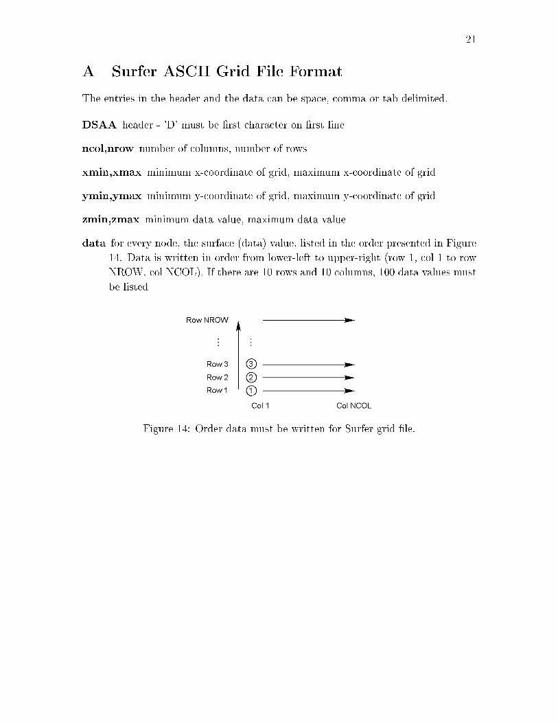
21
A Surfer ASCII Grid File Format
The entries in the header and the data can be space, comma or tab delimited.
DSAA header - 'D' must be �rst character on �rst line
ncol,nrow number of columns, number of rows
xmin,xmax minimum x-coordinate of grid, maximum x-coordinate of grid
ymin,ymax minimum y-coordinate of grid, maximum y-coordinate of grid
zmin,zmax minimum data value, maximum data value
data for every node, the surface (data) value, listed in the order presented in Figure
14. Data is written in order from lower-left to upper-right (row 1, col 1 to row
NROW, col NCOL). If there are 10 rows and 10 columns, 100 data values must
be listed
Figure 14: Order data must be written for Surfer grid �le.