ordinary kriging r
DESCRIPTION
Ordinary Kriging in RTRANSCRIPT

University of California, Los AngelesDepartment of Statistics
Statistics C173/C273 Instructor: Nicolas Christou
Ordinary kriging using geoR and gstat
In this document we will discuss kriging using the R packages geoR and gstat. We will usethe numerical example from last lecture. Here it is:
A simple example:Consider the following data
si x y z(si)s1 61 139 477s2 63 140 696s3 64 129 227s4 68 128 646s5 71 140 606s6 73 141 791s7 75 128 783s0 65 137 ???
Our goal is to estimate the unknown value at location s0. Here is the x− y plot:
●
●
●
●
●
●
●
●
62 64 66 68 70 72 74
128
130
132
134
136
138
140
x coordinate
y co
ordi
nate
s0
s1s2
s3s4
s5s6
s7
1

For these data, let’s assume that we use the exponential semivariogram model with param-eters c0 = 0, c1 = 10, α = 3.33.
γ(h) = c0 + c1(1− e−hα ) = 10(1− e−
h3.33 ).
which is equivalent to the covariance function
C(h) =
{c0 + c1, h = 0
c1e− hα , h > 0
⇒ C(h) =
{10, h = 0
10e−h
3.33 , h > 0
The predicted value at location s0 is equal to:
z(s0) =n∑
i=1
wiz(si) = 0.174(477) + · · ·+ 0.086(783) = 592.59.
And the variance:
σ2e =
n∑i=1
wiγ(si − s0) + λ = 0.174(7.384) + · · ·+ 0.086(9.823) + 0.906 = 8.96.
Kriging using geoR:We will use now the geoR package to find the same result. First we read our data as ageodata object:
> a <- read.table("http://www.stat.ucla.edu/~nchristo/statistics_c173_c273/
kriging_11.txt", header=TRUE)
> b <- as.geodata(a)
To predict the unknown value at locaton (x = 65, y = 137) we use the following:
> prediction <- ksline(b, cov.model="exp", cov.pars=c(10,3.33), nugget=0,
locations=c(65,137))
where,b The geodatacov.model The model we are usingcov.pars The parameters of the model (partial sill and range)nugget The value of the nugget effectlocations The coordinates (x, y) of the points to be predicted
The object “prediction” contains among other things the predicted value at location x =65, y = 137 and its variance. We can obtain them as follows:
> prediction$predict
[1] 592.7587
> prediction$krige.var
[1] 8.960294
2

Suppose now we want to predict the value at many locations. The following commands willproduce a grid whose points will be estimated using kriging:
> x <- seq(61, 75, by=1)
> y <- seq(128,141, by=1)
> xv <- rep(x,14)
> yv <- rep(y, each=15)
> in_mat <- as.matrix(cbind(xv,yv))
Of course the matrix can be constructed also as follows:
> x.range <- as.integer(range(a[,1]))
> y.range <- as.integer(range(a[,2]))
> x=seq(from=x.range[1], to=x.range[2], by=1)
> y=seq(from=y.range[1], to=y.range[2], by=1)
> length(x)
> length(y)
> xv <- rep(x,length(y))
> yv <- rep(y, each=length(x))
> in_mat <- as.matrix(cbind(xv,yv))
> plot(in_mat)
This grid consists of 15× 14 = 210 points stored in the matrix in mat. The command thatpredicts the value at each one of these points is the following:
> q <- ksline(b, cov.model="exp",cov.pars=c(10,3.33), nugget=0,
locations=in_mat)
ksline: kriging location: 1 out of 210
ksline: kriging location: 101 out of 210
ksline: kriging location: 201 out of 210
ksline: kriging location: 210 out of 210
Kriging performed using global neighbourhood
We can access the predicted values and their variances using q$predict and q$krige.var.Here are the first 5 predicted values with their variances:
> cbind(q$predict[1:5], q$krige.var[1:5])
[,1] [,2]
[1,] 458.4491 9.245493
[2,] 413.2103 7.850838
[3,] 362.4674 5.927999
[4,] 338.9828 4.516906
[5,] 393.3933 5.280417
3

To construct the raster map we type:
image(q, val=q$predict)
Or simply:
image(q)
Here is the plot:
65 70 75
128
130
132
134
136
138
140
X Coord
Y C
oord
And here is the plot with the data points:
points(a)
65 70 75
128
130
132
134
136
138
140
X Coord
Y Co
ord
●
●
●
●
●
●
●
4
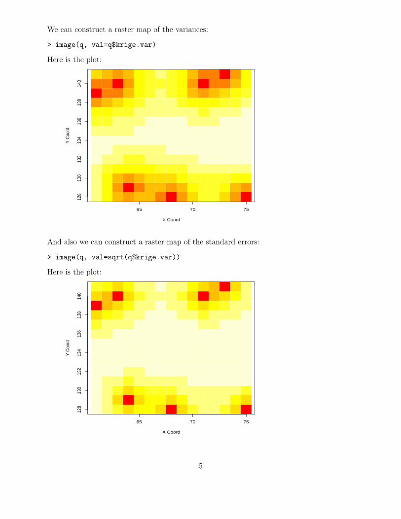
We can construct a raster map of the variances:
> image(q, val=q$krige.var)
Here is the plot:
65 70 75
128
130
132
134
136
138
140
X Coord
Y C
oord
And also we can construct a raster map of the standard errors:
> image(q, val=sqrt(q$krige.var))
Here is the plot:
65 70 75
128
130
132
134
136
138
140
X Coord
Y C
oord
5

The following command will construct a perspective plot of the predicted values:
> persp(x,y,matrix(q$predict,15,14), xlab="x coordinate",
ylab="y coordinate", zlab="Predicted values of z",
main="Perspective plot of the predicted values")
x coordinate
ycoo
rdin
ate
Predictedvalues ofz
Perspective plot of the predicted values
And here is the perspective plot of the standard errors:
> persp(x,y,matrix(sqrt(q$krige.var),15,14), xlab="x coordinate",
ylab="ycoordinate", zlab="Predicted values of z",
main="Perspective plot of the standard errors")
x coordinate
ycoo
rdin
ate
Predicted values of z
Perspective plot of the standard errors
6

Commnets:The argument locations for the function ksline can be a matrix or a data frame. So farwe use a matrix (in mat). We can also use a data frame as follows:
> x.range <- as.integer(range(a[,1]))
> y.range <- as.integer(range(a[,2]))
> grd <- expand.grid(x=seq(from=x.range[1], to=x.range[2], by=1),
y=seq(from=y.range[1], to=y.range[2], by=1))
> q <- ksline(b, cov.model="exp",cov.pars=c(10,3.33), nugget=0,
locations=grd)
Another function in geoR that performs kriging is the krige.conv function. It can be usedas follows:
> kc <- krige.conv(b, loc=in_mat,
krige=krige.control(cov.pars=c(10, 3.33), nugget=0))
krige.conv: model with constant mean
krige.conv: Kriging performed using global neighbourhood
Or using a data frame argument for locations:
> kc <- krige.conv(b, loc=grd,
krige=krige.control(cov.pars=c(10, 3.33), nugget=0))
krige.conv: model with constant mean
krige.conv: Kriging performed using global neighbourhood
In case you have a variofit output you can use it as an input of the argument krige asfollows (this is only an example):
var1 <- variog(b, max.dist=1000)
fit1 <- variofit(var1, cov.model="exp", ini.cov.pars=c(1000, 100),
fix.nugget=FALSE, nugget=250)
qq <- krige.conv(b, locations=grd, krige=krige.control(obj.model=fit1))
7

Kriging using gstat:We will use now the gstat package to find the same result. First we read our data andcreate the grid for prediction as follows:
> a <- read.table("http://www.stat.ucla.edu/~nchristo/statistics_c173_c273/
kriging_11.txt", header=TRUE)
> x.range <- as.integer(range(a[,1]))
> y.range <- as.integer(range(a[,2]))
> grd <- expand.grid(x=seq(from=x.range[1], to=x.range[2], by=1),
y=seq(from=y.range[1], to=y.range[2], by=1))
We now define the model. Normally the model must be estimated from the sample variogram,but for this simple example we assume that it is given as below:
> library(gstat)
> m <- vgm(10, "Exp", 3.33, 0)
There are two ways to perform ordinary kriging with gstat. The data and the grid are usedas data frames, with the extra argument locations as shown below:
> q1 <- krige(id="z", formula=z~1, data=a, newdata=grd, model = m,
locations=~x+y)
The other way is to convert the data and the grid as spatial data points data frame:
> coordinates(a) <- ~x+y
> coordinates(grd) <- ~x+y
> q2 <- krige(id="z", formula=z~1, a, newdata=grd, model = m)
Important note: If we use the second way the argument data= is not allowed. We simply usethe name of the data, here just a. Also, q1 is a data frame, while q2 is spatial data pointsdata frame. Using q1 we can create a 3D plot with the libraries scatterploted and rgl asfollows:
> library(scatterplot3d)
> library(rgl)
> scatterplot3d(q1$x, q1$y, q1$z.pred, xlab="x", ylab="y",
zlab="Predicted values")
> plot3d(q1$x, q1$y, q1$z.pred, size=3)
8

Here are the plots:(a). Using the scatterplot3d command.
60 62 64 66 68 70 72 74 76
20
03
00
40
05
00
60
07
00
80
0
128
130
132
134
136
138
140
142
x
y
Pre
dic
ted
va
lue
s
●
●
●
●
●●●●●●
●●●
●
●
●●●
●
●●●●●●●
●
●
●
●
●●●
●
●●●●●●●●
●
●
●
●●●●
●●●●●●●●
●
●
●
●●●●
●●●●●●●●●
●●
●●●●●●●●●●●●●
●●
●●●●●●
●●
●●
●●●●●
●●●●●●
●●
●●
●●●●●
●●●●●
●●
●●
●●
●●●●
●●●●
●●
●
●
●
●
●●●
●●
●●●
●●
●●
●
●
●
●
●●
●
●
●●●
●●
●●
●
●
●
●
●
●
●
●
●●
●●
●●
●
●
●
●
●
●
●
●
●
●
●
●●
●●●●
●
●
●
●●
●
●
(b). Using the plot3d command.
9

A complete example on kriging using gstat:We will use again the soil data from the Maas river. Here is some background.The actual data set contains many variables but here we will use the x, y coordinates andthe concentration of lead and zinc in ppm at each data point. The motivation for this studyis to predict the concentration of heavy metals around the banks of the Maas river in thearea west of the town Stein in the Netherlands. These heavy metals were accumulated overthe years because of river pollution. Here is the area of study:
10

You can access the data at
> a <- read.table("http://www.stat.ucla.edu/~nchristo/statistics_c173_c273/
soil.txt", header=TRUE)
# Save the original image function:
> image.orig <- image
To load the gstat package type
> library(gstat)
First, we will compute the descriptive statistics of the data set, construct the stem-and-leafplots, histograms, and boxplots:
> stem(a$lead)
> boxplot(a$lead)
> hist(a$lead)
> stem(a$zinc)
> boxplot(a$zinc)
> hist(a$zinc)
> summary(a)
Transform the data (logarithm transformation):
> log_lead <- log10(a$lead)
> log_zinc <- log10(a$zinc)
> stem(log_lead)
> boxplot(log_lead)
> hist(log_lead)
> stem(log_zinc)
> boxplot(log_zinc)
> hist(log_zinc)
#Create a gstat object;
> g <- gstat(id="log_lead", formula = log(lead)~1, locations = ~x+y,
data = a)
#Plot the variogram:
> plot(variogram(g), main="Semivariogram of the log_lead")
#Fit a model variogram to the sample variogram:
> v.fit <- fit.variogram(variogram(g), vgm(0.5,"Sph",1000,0.1))
> plot(variogram(g),v.fit)
#Note: The values above were the initial values for the partial sill,
#range, and nugget. Then the function fit.variogram uses a minimization
#procedure to fit a model variogram to the sample variogram. Type v.fit
11

#to get the estimates of the model parameters.
> v.fit
model psill range
1 Nug 0.05156252 0.0000
2 Sph 0.51530678 965.1506
#There are different weights you can use in the minimization procedure. The
#default (the one used above) is $N_h/h^2$ where $N_h$ is the number of pairs
#and $h$ the separation distance. You can chose the type of weights by using
#the argument fit.method=integer, where integer is a number from the table
#below:
fit.method weights
1 N_h
2 N_h/gamma(h;theta)^2 (Cressie’s weights)
6 OLS (no weights)
7 N_h/h^2 (default)
#Use kriging to estimate the value of log(lead) at the grid values.
#First we create the grid.
> x.range <- as.integer(range(a[,1]))
> x.range
> y.range <- as.integer(range(a[,2]))
> y.range
> grd <- expand.grid(x=seq(from=x.range[1], to=x.range[2], by=50),
y=seq(from=y.range[1], to=y.range[2], by=50))
#We want now to use kriging to predict log(lead) at each point on the grid:
> pr_ok <- krige(id="log_lead",log(lead)~1, locations=~x+y,
model=v.fit,
data=a, newdata=grd)
#To find what the object pr_ok contains type:
> names(pr_ok)
[1] "x" "y" "log_lead.pred" "log_lead.var"
#To see the predicted values you type:
> pr_ok$log_lead.pred
#And the kriging variances:
> pr_ok$log_lead.var
12

The plot of the sample variogram:
> plot(variogram(g), main="Semivariogram of the log_lead")
Semivariogram of the log_lead
distance
sem
ivaria
nce
0.1
0.2
0.3
0.4
0.5
0.6
500 1000 1500
●
●
●
●
●
●
●
●
●
●
●
●
●
●●
The fitted spherical variogram to the sample variogram:
> plot(variogram(g),v.fit)
Fitted spherical semivariogram
distance
sem
ivaria
nce
0.1
0.2
0.3
0.4
0.5
0.6
500 1000 1500
●
●
●
●
●
●
●
●
●
●
●
●
●
●●
13

Here is the grid for the kriging predictions:
> plot(grd)
● ● ● ● ● ● ● ● ● ● ● ● ● ● ● ● ● ● ● ● ● ● ● ● ● ● ● ● ● ● ● ● ● ● ● ● ● ● ● ● ● ● ● ● ● ● ● ● ● ● ● ● ● ● ● ●● ● ● ● ● ● ● ● ● ● ● ● ● ● ● ● ● ● ● ● ● ● ● ● ● ● ● ● ● ● ● ● ● ● ● ● ● ● ● ● ● ● ● ● ● ● ● ● ● ● ● ● ● ● ● ●● ● ● ● ● ● ● ● ● ● ● ● ● ● ● ● ● ● ● ● ● ● ● ● ● ● ● ● ● ● ● ● ● ● ● ● ● ● ● ● ● ● ● ● ● ● ● ● ● ● ● ● ● ● ● ●● ● ● ● ● ● ● ● ● ● ● ● ● ● ● ● ● ● ● ● ● ● ● ● ● ● ● ● ● ● ● ● ● ● ● ● ● ● ● ● ● ● ● ● ● ● ● ● ● ● ● ● ● ● ● ●● ● ● ● ● ● ● ● ● ● ● ● ● ● ● ● ● ● ● ● ● ● ● ● ● ● ● ● ● ● ● ● ● ● ● ● ● ● ● ● ● ● ● ● ● ● ● ● ● ● ● ● ● ● ● ●● ● ● ● ● ● ● ● ● ● ● ● ● ● ● ● ● ● ● ● ● ● ● ● ● ● ● ● ● ● ● ● ● ● ● ● ● ● ● ● ● ● ● ● ● ● ● ● ● ● ● ● ● ● ● ●● ● ● ● ● ● ● ● ● ● ● ● ● ● ● ● ● ● ● ● ● ● ● ● ● ● ● ● ● ● ● ● ● ● ● ● ● ● ● ● ● ● ● ● ● ● ● ● ● ● ● ● ● ● ● ●● ● ● ● ● ● ● ● ● ● ● ● ● ● ● ● ● ● ● ● ● ● ● ● ● ● ● ● ● ● ● ● ● ● ● ● ● ● ● ● ● ● ● ● ● ● ● ● ● ● ● ● ● ● ● ●● ● ● ● ● ● ● ● ● ● ● ● ● ● ● ● ● ● ● ● ● ● ● ● ● ● ● ● ● ● ● ● ● ● ● ● ● ● ● ● ● ● ● ● ● ● ● ● ● ● ● ● ● ● ● ●● ● ● ● ● ● ● ● ● ● ● ● ● ● ● ● ● ● ● ● ● ● ● ● ● ● ● ● ● ● ● ● ● ● ● ● ● ● ● ● ● ● ● ● ● ● ● ● ● ● ● ● ● ● ● ●● ● ● ● ● ● ● ● ● ● ● ● ● ● ● ● ● ● ● ● ● ● ● ● ● ● ● ● ● ● ● ● ● ● ● ● ● ● ● ● ● ● ● ● ● ● ● ● ● ● ● ● ● ● ● ●● ● ● ● ● ● ● ● ● ● ● ● ● ● ● ● ● ● ● ● ● ● ● ● ● ● ● ● ● ● ● ● ● ● ● ● ● ● ● ● ● ● ● ● ● ● ● ● ● ● ● ● ● ● ● ●● ● ● ● ● ● ● ● ● ● ● ● ● ● ● ● ● ● ● ● ● ● ● ● ● ● ● ● ● ● ● ● ● ● ● ● ● ● ● ● ● ● ● ● ● ● ● ● ● ● ● ● ● ● ● ●● ● ● ● ● ● ● ● ● ● ● ● ● ● ● ● ● ● ● ● ● ● ● ● ● ● ● ● ● ● ● ● ● ● ● ● ● ● ● ● ● ● ● ● ● ● ● ● ● ● ● ● ● ● ● ●● ● ● ● ● ● ● ● ● ● ● ● ● ● ● ● ● ● ● ● ● ● ● ● ● ● ● ● ● ● ● ● ● ● ● ● ● ● ● ● ● ● ● ● ● ● ● ● ● ● ● ● ● ● ● ●● ● ● ● ● ● ● ● ● ● ● ● ● ● ● ● ● ● ● ● ● ● ● ● ● ● ● ● ● ● ● ● ● ● ● ● ● ● ● ● ● ● ● ● ● ● ● ● ● ● ● ● ● ● ● ●● ● ● ● ● ● ● ● ● ● ● ● ● ● ● ● ● ● ● ● ● ● ● ● ● ● ● ● ● ● ● ● ● ● ● ● ● ● ● ● ● ● ● ● ● ● ● ● ● ● ● ● ● ● ● ●● ● ● ● ● ● ● ● ● ● ● ● ● ● ● ● ● ● ● ● ● ● ● ● ● ● ● ● ● ● ● ● ● ● ● ● ● ● ● ● ● ● ● ● ● ● ● ● ● ● ● ● ● ● ● ●● ● ● ● ● ● ● ● ● ● ● ● ● ● ● ● ● ● ● ● ● ● ● ● ● ● ● ● ● ● ● ● ● ● ● ● ● ● ● ● ● ● ● ● ● ● ● ● ● ● ● ● ● ● ● ●● ● ● ● ● ● ● ● ● ● ● ● ● ● ● ● ● ● ● ● ● ● ● ● ● ● ● ● ● ● ● ● ● ● ● ● ● ● ● ● ● ● ● ● ● ● ● ● ● ● ● ● ● ● ● ●● ● ● ● ● ● ● ● ● ● ● ● ● ● ● ● ● ● ● ● ● ● ● ● ● ● ● ● ● ● ● ● ● ● ● ● ● ● ● ● ● ● ● ● ● ● ● ● ● ● ● ● ● ● ● ●● ● ● ● ● ● ● ● ● ● ● ● ● ● ● ● ● ● ● ● ● ● ● ● ● ● ● ● ● ● ● ● ● ● ● ● ● ● ● ● ● ● ● ● ● ● ● ● ● ● ● ● ● ● ● ●● ● ● ● ● ● ● ● ● ● ● ● ● ● ● ● ● ● ● ● ● ● ● ● ● ● ● ● ● ● ● ● ● ● ● ● ● ● ● ● ● ● ● ● ● ● ● ● ● ● ● ● ● ● ● ●● ● ● ● ● ● ● ● ● ● ● ● ● ● ● ● ● ● ● ● ● ● ● ● ● ● ● ● ● ● ● ● ● ● ● ● ● ● ● ● ● ● ● ● ● ● ● ● ● ● ● ● ● ● ● ●● ● ● ● ● ● ● ● ● ● ● ● ● ● ● ● ● ● ● ● ● ● ● ● ● ● ● ● ● ● ● ● ● ● ● ● ● ● ● ● ● ● ● ● ● ● ● ● ● ● ● ● ● ● ● ●● ● ● ● ● ● ● ● ● ● ● ● ● ● ● ● ● ● ● ● ● ● ● ● ● ● ● ● ● ● ● ● ● ● ● ● ● ● ● ● ● ● ● ● ● ● ● ● ● ● ● ● ● ● ● ●● ● ● ● ● ● ● ● ● ● ● ● ● ● ● ● ● ● ● ● ● ● ● ● ● ● ● ● ● ● ● ● ● ● ● ● ● ● ● ● ● ● ● ● ● ● ● ● ● ● ● ● ● ● ● ●● ● ● ● ● ● ● ● ● ● ● ● ● ● ● ● ● ● ● ● ● ● ● ● ● ● ● ● ● ● ● ● ● ● ● ● ● ● ● ● ● ● ● ● ● ● ● ● ● ● ● ● ● ● ● ●● ● ● ● ● ● ● ● ● ● ● ● ● ● ● ● ● ● ● ● ● ● ● ● ● ● ● ● ● ● ● ● ● ● ● ● ● ● ● ● ● ● ● ● ● ● ● ● ● ● ● ● ● ● ● ●● ● ● ● ● ● ● ● ● ● ● ● ● ● ● ● ● ● ● ● ● ● ● ● ● ● ● ● ● ● ● ● ● ● ● ● ● ● ● ● ● ● ● ● ● ● ● ● ● ● ● ● ● ● ● ●● ● ● ● ● ● ● ● ● ● ● ● ● ● ● ● ● ● ● ● ● ● ● ● ● ● ● ● ● ● ● ● ● ● ● ● ● ● ● ● ● ● ● ● ● ● ● ● ● ● ● ● ● ● ● ●● ● ● ● ● ● ● ● ● ● ● ● ● ● ● ● ● ● ● ● ● ● ● ● ● ● ● ● ● ● ● ● ● ● ● ● ● ● ● ● ● ● ● ● ● ● ● ● ● ● ● ● ● ● ● ●● ● ● ● ● ● ● ● ● ● ● ● ● ● ● ● ● ● ● ● ● ● ● ● ● ● ● ● ● ● ● ● ● ● ● ● ● ● ● ● ● ● ● ● ● ● ● ● ● ● ● ● ● ● ● ●● ● ● ● ● ● ● ● ● ● ● ● ● ● ● ● ● ● ● ● ● ● ● ● ● ● ● ● ● ● ● ● ● ● ● ● ● ● ● ● ● ● ● ● ● ● ● ● ● ● ● ● ● ● ● ●● ● ● ● ● ● ● ● ● ● ● ● ● ● ● ● ● ● ● ● ● ● ● ● ● ● ● ● ● ● ● ● ● ● ● ● ● ● ● ● ● ● ● ● ● ● ● ● ● ● ● ● ● ● ● ●● ● ● ● ● ● ● ● ● ● ● ● ● ● ● ● ● ● ● ● ● ● ● ● ● ● ● ● ● ● ● ● ● ● ● ● ● ● ● ● ● ● ● ● ● ● ● ● ● ● ● ● ● ● ● ●● ● ● ● ● ● ● ● ● ● ● ● ● ● ● ● ● ● ● ● ● ● ● ● ● ● ● ● ● ● ● ● ● ● ● ● ● ● ● ● ● ● ● ● ● ● ● ● ● ● ● ● ● ● ● ●● ● ● ● ● ● ● ● ● ● ● ● ● ● ● ● ● ● ● ● ● ● ● ● ● ● ● ● ● ● ● ● ● ● ● ● ● ● ● ● ● ● ● ● ● ● ● ● ● ● ● ● ● ● ● ●● ● ● ● ● ● ● ● ● ● ● ● ● ● ● ● ● ● ● ● ● ● ● ● ● ● ● ● ● ● ● ● ● ● ● ● ● ● ● ● ● ● ● ● ● ● ● ● ● ● ● ● ● ● ● ●● ● ● ● ● ● ● ● ● ● ● ● ● ● ● ● ● ● ● ● ● ● ● ● ● ● ● ● ● ● ● ● ● ● ● ● ● ● ● ● ● ● ● ● ● ● ● ● ● ● ● ● ● ● ● ●● ● ● ● ● ● ● ● ● ● ● ● ● ● ● ● ● ● ● ● ● ● ● ● ● ● ● ● ● ● ● ● ● ● ● ● ● ● ● ● ● ● ● ● ● ● ● ● ● ● ● ● ● ● ● ●● ● ● ● ● ● ● ● ● ● ● ● ● ● ● ● ● ● ● ● ● ● ● ● ● ● ● ● ● ● ● ● ● ● ● ● ● ● ● ● ● ● ● ● ● ● ● ● ● ● ● ● ● ● ● ●● ● ● ● ● ● ● ● ● ● ● ● ● ● ● ● ● ● ● ● ● ● ● ● ● ● ● ● ● ● ● ● ● ● ● ● ● ● ● ● ● ● ● ● ● ● ● ● ● ● ● ● ● ● ● ●● ● ● ● ● ● ● ● ● ● ● ● ● ● ● ● ● ● ● ● ● ● ● ● ● ● ● ● ● ● ● ● ● ● ● ● ● ● ● ● ● ● ● ● ● ● ● ● ● ● ● ● ● ● ● ●● ● ● ● ● ● ● ● ● ● ● ● ● ● ● ● ● ● ● ● ● ● ● ● ● ● ● ● ● ● ● ● ● ● ● ● ● ● ● ● ● ● ● ● ● ● ● ● ● ● ● ● ● ● ● ●● ● ● ● ● ● ● ● ● ● ● ● ● ● ● ● ● ● ● ● ● ● ● ● ● ● ● ● ● ● ● ● ● ● ● ● ● ● ● ● ● ● ● ● ● ● ● ● ● ● ● ● ● ● ● ●● ● ● ● ● ● ● ● ● ● ● ● ● ● ● ● ● ● ● ● ● ● ● ● ● ● ● ● ● ● ● ● ● ● ● ● ● ● ● ● ● ● ● ● ● ● ● ● ● ● ● ● ● ● ● ●● ● ● ● ● ● ● ● ● ● ● ● ● ● ● ● ● ● ● ● ● ● ● ● ● ● ● ● ● ● ● ● ● ● ● ● ● ● ● ● ● ● ● ● ● ● ● ● ● ● ● ● ● ● ● ●● ● ● ● ● ● ● ● ● ● ● ● ● ● ● ● ● ● ● ● ● ● ● ● ● ● ● ● ● ● ● ● ● ● ● ● ● ● ● ● ● ● ● ● ● ● ● ● ● ● ● ● ● ● ● ●● ● ● ● ● ● ● ● ● ● ● ● ● ● ● ● ● ● ● ● ● ● ● ● ● ● ● ● ● ● ● ● ● ● ● ● ● ● ● ● ● ● ● ● ● ● ● ● ● ● ● ● ● ● ● ●● ● ● ● ● ● ● ● ● ● ● ● ● ● ● ● ● ● ● ● ● ● ● ● ● ● ● ● ● ● ● ● ● ● ● ● ● ● ● ● ● ● ● ● ● ● ● ● ● ● ● ● ● ● ● ●● ● ● ● ● ● ● ● ● ● ● ● ● ● ● ● ● ● ● ● ● ● ● ● ● ● ● ● ● ● ● ● ● ● ● ● ● ● ● ● ● ● ● ● ● ● ● ● ● ● ● ● ● ● ● ●● ● ● ● ● ● ● ● ● ● ● ● ● ● ● ● ● ● ● ● ● ● ● ● ● ● ● ● ● ● ● ● ● ● ● ● ● ● ● ● ● ● ● ● ● ● ● ● ● ● ● ● ● ● ● ●● ● ● ● ● ● ● ● ● ● ● ● ● ● ● ● ● ● ● ● ● ● ● ● ● ● ● ● ● ● ● ● ● ● ● ● ● ● ● ● ● ● ● ● ● ● ● ● ● ● ● ● ● ● ● ●● ● ● ● ● ● ● ● ● ● ● ● ● ● ● ● ● ● ● ● ● ● ● ● ● ● ● ● ● ● ● ● ● ● ● ● ● ● ● ● ● ● ● ● ● ● ● ● ● ● ● ● ● ● ● ●● ● ● ● ● ● ● ● ● ● ● ● ● ● ● ● ● ● ● ● ● ● ● ● ● ● ● ● ● ● ● ● ● ● ● ● ● ● ● ● ● ● ● ● ● ● ● ● ● ● ● ● ● ● ● ●● ● ● ● ● ● ● ● ● ● ● ● ● ● ● ● ● ● ● ● ● ● ● ● ● ● ● ● ● ● ● ● ● ● ● ● ● ● ● ● ● ● ● ● ● ● ● ● ● ● ● ● ● ● ● ●● ● ● ● ● ● ● ● ● ● ● ● ● ● ● ● ● ● ● ● ● ● ● ● ● ● ● ● ● ● ● ● ● ● ● ● ● ● ● ● ● ● ● ● ● ● ● ● ● ● ● ● ● ● ● ●● ● ● ● ● ● ● ● ● ● ● ● ● ● ● ● ● ● ● ● ● ● ● ● ● ● ● ● ● ● ● ● ● ● ● ● ● ● ● ● ● ● ● ● ● ● ● ● ● ● ● ● ● ● ● ●● ● ● ● ● ● ● ● ● ● ● ● ● ● ● ● ● ● ● ● ● ● ● ● ● ● ● ● ● ● ● ● ● ● ● ● ● ● ● ● ● ● ● ● ● ● ● ● ● ● ● ● ● ● ● ●● ● ● ● ● ● ● ● ● ● ● ● ● ● ● ● ● ● ● ● ● ● ● ● ● ● ● ● ● ● ● ● ● ● ● ● ● ● ● ● ● ● ● ● ● ● ● ● ● ● ● ● ● ● ● ●● ● ● ● ● ● ● ● ● ● ● ● ● ● ● ● ● ● ● ● ● ● ● ● ● ● ● ● ● ● ● ● ● ● ● ● ● ● ● ● ● ● ● ● ● ● ● ● ● ● ● ● ● ● ● ●● ● ● ● ● ● ● ● ● ● ● ● ● ● ● ● ● ● ● ● ● ● ● ● ● ● ● ● ● ● ● ● ● ● ● ● ● ● ● ● ● ● ● ● ● ● ● ● ● ● ● ● ● ● ● ●● ● ● ● ● ● ● ● ● ● ● ● ● ● ● ● ● ● ● ● ● ● ● ● ● ● ● ● ● ● ● ● ● ● ● ● ● ● ● ● ● ● ● ● ● ● ● ● ● ● ● ● ● ● ● ●● ● ● ● ● ● ● ● ● ● ● ● ● ● ● ● ● ● ● ● ● ● ● ● ● ● ● ● ● ● ● ● ● ● ● ● ● ● ● ● ● ● ● ● ● ● ● ● ● ● ● ● ● ● ● ●● ● ● ● ● ● ● ● ● ● ● ● ● ● ● ● ● ● ● ● ● ● ● ● ● ● ● ● ● ● ● ● ● ● ● ● ● ● ● ● ● ● ● ● ● ● ● ● ● ● ● ● ● ● ● ●● ● ● ● ● ● ● ● ● ● ● ● ● ● ● ● ● ● ● ● ● ● ● ● ● ● ● ● ● ● ● ● ● ● ● ● ● ● ● ● ● ● ● ● ● ● ● ● ● ● ● ● ● ● ● ●● ● ● ● ● ● ● ● ● ● ● ● ● ● ● ● ● ● ● ● ● ● ● ● ● ● ● ● ● ● ● ● ● ● ● ● ● ● ● ● ● ● ● ● ● ● ● ● ● ● ● ● ● ● ● ●● ● ● ● ● ● ● ● ● ● ● ● ● ● ● ● ● ● ● ● ● ● ● ● ● ● ● ● ● ● ● ● ● ● ● ● ● ● ● ● ● ● ● ● ● ● ● ● ● ● ● ● ● ● ● ●● ● ● ● ● ● ● ● ● ● ● ● ● ● ● ● ● ● ● ● ● ● ● ● ● ● ● ● ● ● ● ● ● ● ● ● ● ● ● ● ● ● ● ● ● ● ● ● ● ● ● ● ● ● ● ●● ● ● ● ● ● ● ● ● ● ● ● ● ● ● ● ● ● ● ● ● ● ● ● ● ● ● ● ● ● ● ● ● ● ● ● ● ● ● ● ● ● ● ● ● ● ● ● ● ● ● ● ● ● ● ●● ● ● ● ● ● ● ● ● ● ● ● ● ● ● ● ● ● ● ● ● ● ● ● ● ● ● ● ● ● ● ● ● ● ● ● ● ● ● ● ● ● ● ● ● ● ● ● ● ● ● ● ● ● ● ●● ● ● ● ● ● ● ● ● ● ● ● ● ● ● ● ● ● ● ● ● ● ● ● ● ● ● ● ● ● ● ● ● ● ● ● ● ● ● ● ● ● ● ● ● ● ● ● ● ● ● ● ● ● ● ●● ● ● ● ● ● ● ● ● ● ● ● ● ● ● ● ● ● ● ● ● ● ● ● ● ● ● ● ● ● ● ● ● ● ● ● ● ● ● ● ● ● ● ● ● ● ● ● ● ● ● ● ● ● ● ●● ● ● ● ● ● ● ● ● ● ● ● ● ● ● ● ● ● ● ● ● ● ● ● ● ● ● ● ● ● ● ● ● ● ● ● ● ● ● ● ● ● ● ● ● ● ● ● ● ● ● ● ● ● ● ●● ● ● ● ● ● ● ● ● ● ● ● ● ● ● ● ● ● ● ● ● ● ● ● ● ● ● ● ● ● ● ● ● ● ● ● ● ● ● ● ● ● ● ● ● ● ● ● ● ● ● ● ● ● ● ●● ● ● ● ● ● ● ● ● ● ● ● ● ● ● ● ● ● ● ● ● ● ● ● ● ● ● ● ● ● ● ● ● ● ● ● ● ● ● ● ● ● ● ● ● ● ● ● ● ● ● ● ● ● ● ●● ● ● ● ● ● ● ● ● ● ● ● ● ● ● ● ● ● ● ● ● ● ● ● ● ● ● ● ● ● ● ● ● ● ● ● ● ● ● ● ● ● ● ● ● ● ● ● ● ● ● ● ● ● ● ●
178500 179000 179500 180000 180500 181000
3300
0033
1000
3320
0033
3000
Grid for the kriging predictions
x
y
Load the library scatterplot3d:
> library(scatterplot3d)
> scatterplot3d(pr_ok$x, pr_ok$y, pr_ok$log_lead.pred, main="Predicted values")
Predicted values
178500 179000 179500 180000 180500 181000 181500
3.5
4.0
4.5
5.0
5.5
6.0
6.5
329000
330000
331000
332000
333000
334000
pr_ok$x
pr_o
k$y
pr_o
k$log
_lead
.pre
d
●●
●
●
●
●●
●●●●●●●●●
●●
●●
●●
●●●●●●●●●●●●●●●●●●●●●●●●●●●●●●●●●●
●●●
●
●
●●
●●●●●●●●
●●
●●
●●
●●
●●●●●●●●●●●●●●●●●●●●●●●●●●●●●●●●●
●●●
●●
●●
●●
●●●●●●●
●●
●●
●●
●●
●●●●●●●●●●●●●●●●●●●●●●●●●●●●●●●●
●●●●
●●
●
●
●
●●●●●●
●●
●●
●●
●●
●●●●●●●●●●●●●●●●●●●●●●●●●●●●●●●●●
●●●●●
●●
●
●
●●●●●●●●●●●
●●
●●●●●●●●●●●●●●●●●●●●●●●●●●●●●●●●●●
●●●●●
●●
●
●
●●●●●●●●●●●●
●●
●●●●●●●●●●●●●●●●●●●●●●●●●●●●●●●●●
●●●●
●●
●
●
●
●●●●●●●●●●●●
●●
●●●●●●●●●●●●●●●●●●●●●●●●●●●●●●●●●
●●●●
●●
●
●
●●
●●●●●●●●●●●●●
●●●●●●●●●●●●●●●●●●●●●●●●●●●●●●●●●
●●
●●●
●●
●●
●●●●●
●●●●●●●●●●●●●●●●●●●●●●●●●●●●●●●●●●●●●●●●●●
●●●●●
●●
●●
●●●●
●●
●●●●●●●●●●●●●●●●●●●●●●●●●●●●●●●●●●●●●●●●●
●●●●●
●●
●●
●●●
●●
●●
●●●●●●●●●●●●●●●●●●●●●●●●●●●●●●●●●●●●●●●●
●●●●●
●●
●●
●●
●●
●●
●●
●●●●●●●●●●●●●●●●●●●●●●●●●●●●●●●●●●●●●●●
●●●●
●●●●
●●
●●
●●
●●
●●
●●●●●●●●●●●●
●●
●●●●●●●●●●●●●●●●●●●●●●●●
●●●●
●●●●●●
●
●
●
●
●
●●
●●●●●●●●●●●●
●●
●●
●●●●●●●●●●●●●●●●●●●●●●●
●●●●●●●●●●
●
●
●
●
●
●●
●●
●●●●●●●●●●●
●●
●●
●●●●●●●●●●●●●●●●●●●●●●
●●●●●●●●●●
●
●
●
●
●
●
●●
●●●●●●●●●●●
●●
●●
●●
●●●●●
●●●●●●●●●●●●●●●●
●●●●●●●●●
●●
●
●
●
●
●
●●
●●●●●●●●●●●
●●
●●
●●
●●●●
●●
●●●●●●●●●●●●●●●
●●●●●●●●●●
●●
●
●
●
●
●●
●●
●●●●●●●●●●
●●
●●
●●
●●●
●●
●●
●●●●●●●●●●●●●
●●●●●●●●●●
●●
●
●
●
●
●●
●●
●●
●●●●●●●●
●●
●●
●●
●●●●
●●
●●
●●●●●●●●●●●●
●●●●●●●●●●
●
●
●
●
●
●
●●
●
●●
●●●●●●●●●
●●
●●
●●
●●
●●●
●●
●●●●●●●●●●●●●
●●
●●●●
●●●●●
●
●
●
●
●
●●
●
●
●●●●
●●●●●●
●●
●●
●●
●●
●●●
●●
●●
●●●●●●●●●●●
●●
●●
●●
●●●●●
●
●
●
●
●
●
●
●
●
●●●●
●●
●●●●●
●●
●●
●●
●●●●
●●
●●
●●●●●●●●●●●
●●
●●
●●●●●●●
●
●
●
●
●●
●
●
●
●●●●
●●
●●●●●
●●
●●
●●
●●●●
●●
●●
●●●●●●●●●●●
●●
●●
●●●●●●●
●
●
●
●●
●
●
●
●
●●●●
●
●●
●●●●
●●
●●
●●
●●●●
●●
●●
●●
●●●●●●●●●
●●
●●
●●●●●●●
●●
●●
●●
●
●
●
●●●
●
●
●
●●●●
●●
●●
●●
●●
●●●●●
●●
●●
●●
●●●●●●●
●●
●●
●●●●●●●●
●●●●
●●
●
●
●●●
●
●
●
●●●
●●
●●
●●
●●
●●●●●
●●
●●
●●
●●●●●●●●
●●
●●
●●●●●
●●●●●●●●
●
●
●
●
●●
●
●
●●
●●●
●●
●●
●●
●●
●●●●●
●●
●●
●●
●●●●●●●
●●
●●
●●
●●
●●
●●●●●●●
●
●
●
●
●
●●
●
●●●●●●●●
●●●●
●●●●●●
●●
●●
●●
●●
●●●●●
●●
●●
●●
●●
●●
●●●●●●●
●
●
●
●
●●●●
●●
●●●●●●●●●●●
●●●●●●
●●
●●
●●
●●
●●●●
●●
●●
●●
●●
●●
●●
●●●●●●
●
●
●
●
●●
●
●
●
●●●●
●●●●
●●●
●●●●●●●
●●●
●●
●●
●●●● ●
●●
●●
●●
●●
●●
●●●●●●
●
●
●
●
●●
●
●●
●
●●●
●●●●
●
●●●●●●●●●●●●●●●
●●
●●
●● ●●
●
●●
●●
●●
●●
●●●●●●
●
●
●
●
●●
●
●●●
●●●●
●●●●
●●●●●●●●●●●●●●●●
●●
●●● ●
●●
●
●●
●●
●●
●●
●●●●●●
●
●
●
●●
●●●●●●●●●●●●
●
●●●●●●●●●●●●●●●●
●●
●● ●●
●
●
●●
●●
●●
●●
●●●●●●
●
●
●
●●
●
●●●●●●●●●
●●
●
●
●●●●●●●●●●●●●●●●●
●● ●●●
●
●●
●●
●●
●●
●●●●●●
●
●
●
●●
●
●●●●●●●●●●
●
●
●
●●●●
●●●●●●●●●●●●●●● ●●●
●
●
●●
●●
●●
●●
●●●●●●
●
●
●●
●●
●●●●●●●●●
●
●
●
●●●●
●●●●●●●●●●●●●●● ●●●
●
●
●●
●●
●●
●●
●●●●●●
●
●
●
●●●
●●
●●●●●●●
●
●
●
●●
●●
●●●●●●●●
●●
●●●●● ●●●
●
●
●●
●●
●●
●●
●●●●●●●
●
●
●●●
●●
●●●●●●●●
●
●
●
●●
●●
●●●●●●●●
●●
●●●● ●●●
●
●●
●●
●●
●●
●●●●●●●
●
●
●
●●
●
●
●●
●●●●●●●
●
●
●
●●
●●
●●●●●●●
●●
●●●●●
●●●●
●●
●●
●●
●●
●●
●●●●●●
●
●
●
●●
●
●●
●●●●●●
●●
●
●
●●
●●
●●
●●●●●●
●●
●●●●
●●●●
●●
●●
●●
●●
●●
●●●●●●
●
●
●
●●
●
●●
●●●●●
●●
●●
●
●
●●
●●
●●●●●●
●●
●●
●●●●●●
●●
●●
●●
●●
●●
●●
●●●●●
●●
●●●
●●
●●●●●●
●●
●●
●
●
●●
●●
●●
●●●●●●
●●
●●●
●●●●
●●
●●
●●
●●
●●
●●
●●●
●●
●●●●●
●●
●●●●●●
●
●
●●●
●
●
●●
●●
●●●●●●
●●
●●●
●●●●●
●●
●●
●●
●●
●●
●●
●●●●●●●●●●●●●●●●
●
●
●
●●
●
●
●
●●
●●
●●●●●●
●●
●●●
●●●●●
●●
●●
●●
●●
●●
●●
●●●●●●●●●●●●●●●●
●
●
●
●●●
●
●
●●
●●
●●
●●●●●
●●
●●
●●●●●
●●
●●
●●
●●
●●
●●
●●●●●●●●●●●●●●
●●
●
●
●
●●
●
●
●●
●●●
●●
●●●●●
●●
●●
●●●●●●
●●
●●
●●
●●
●●
●●
●●
●●●●●●●●●●●●●
●
●
●
●
●
●
●
●●●
●●
●●
●●●●●
●●
●●
●●●●●●
●●
●●
●●
●●
●●
●●
●●
●●●●●●●●●●●●●
●
●
●
●
●
●●●●●●
●●
●●
●●●●●
●●
●
●●●●●●●
●●
●●
●●
●●
●●
●●
●●
●●●●
●●●●●●●●●
●
●
●
●
●●●●●●
●●
●●
●●●●●
●●
●
●●●●●●●
●●
●●
●●
●●
●●
●●
●●
●●●●●●●●●●●●●
●
●
●
●
●●
●●●●●
●●
●●●●●●
●●
●
●●●●●●●●
●●
●●
●●
●●●
●●
●●●●●●●●●
●●●●●
●
●
●
●
●
●●●●●
●●
●●
●●●●●●
●●
●
●●●●●●●●
●●
●●
●●
●●●●
●●
●●●●●●●●●
●●●●●
●
●
●
●
●●
●●●
●
●
●●
●●●●●
●●
●●
●●●●●●●●
●●
●●
●●●●●
●●
●●●●●●●●
●●
●●●
●●
●
●
●
●
●
●●
●●
●
●
●
●●
●●●●
●●
●●
●●●●●●●●
●●
●●
●●●●●
●●
●●●●●●●
●●
●
●●●
●
●●
●
●
●
●●
●●
●
●
●
●●
●●●●
●●
●●
●
●●●●●●●●●
●●
●●
●●●●●●
●●●●●●●
●●
●
●
●●
●
●●●
●●
●●●
●
●
●
●
●●●
●●●
●●
●●
●
●●●●●●●●●
●●
●●●●●●●●
●●●●●●●
●●
●
●
●
●
●
●●●●
●●●●●
●
●
●
●●
●●
●●●
●●
●●
●●●●●●●●●●●
●●●●●●●●●
●●●●●●●●
●
●
●
●
●
●●●●●●●●●
●
●
●
●
●●●
●●●●
●●●
●●●●●●●●●●●●●●●●●●●●●●●●●●●●
●
●●
●
●
●●●●●●●●●
●
●
●
●
●●●
●●●●●●●
●●●●●●●●●●●●●●●●●●●●●●●●●●●●●●●●
●●
●●●●●●●●●
●
●
●
●●●●●●●●●●
●●●●●●●●●●●●●●●●●●●●●●●●●●●
●●
●●
●●●●●●●●●●●
●
●
●
●
●●●●●●●
●●●
●●●●●●●●●●●●●●●●●
●●
●●●●●●●●
●
●
●
●
●●●●●●●●●●●
●●
●
●
●
●●●●●
●●●●
●●●●●●●●●●●●●●●●
●●
●●
●●●●●
●
●
●
●
●
●
●●●●●●●●●●●
●●
●
●
●●●●●●●
●●●
●●●●●●●●●●●●●●●●
●●
●●
●●
●●●●
●
●
●
●
●
●●●●●●●●●●●
●●
●
●
●
●●●●●●
●●●
●●●●●●●●●●●●●●●●
●●
●●
●●
●●●
●
●
●
●
●
●
●
●●
●●
●●●●●
●●
●
●
●
●
●●●●●●
●●
●
●●●●●●●●●●●●●●●●
●●
●
●
●
●
●
●●
●
●
●
●
●
●
●
●●
●●
●●●●●
●●
●
●
●
●●●●●●
●●
●●
●●●●●●●●●●●●●●●●
●●
●
●
●
●●
●●
●
●
●
●
●
●
●
●
●●
●●
●●●●●
●
●
●
●
●●●●●●
●●
●●
●●●●●●●●●●●●●●●●
●●
●
●
●●
●●●
●
●
●
●
●
●
●
●
●
●●
●●●●
●●
●●
●
●
●●●●●●
●●
●●
●●●●●●●●●●●●●●●●
●●
●
●●
●●●●
●●
●
●
●
●
●
●
●
●
●●
●●●●
●●●
●
●
●●
●●●
●●
●●●
●●●●●●●●●●●●●●●●
●●
●●
●●●●●●
●●
●
●
●
●
●
●
●
●●
●●●●
●●●●
●
●●
●●
●●
●●
●●
●●●●●●●●●●●●●●
●●
●●
●●
●●●●●●
●●
●
●
●
●
●
●
●
●●
●●●
●●●●
●●
●
●
●
●●
●●
●●●
●●●●●●●●●●●●●●
●●
●●
●●
●●●●●●●
●●
●
●
●
●
●
●●
●●●
●●
●●●●●●●
●
●
●●
●●●●
●●●●●●●●●●●●●●
●●
●●
●●●●●●●●●
●●
●
●
●
●
●
●●
●●●
●●
●●●●●●
●
●
●
●●
●●●●
●●●●●●●●●●●●●●●
●●
●●●●●●●●●●
●●
●●
●
●
●
●
●●
●●
●●
●●●●●●
●
●
●
●●
●●●●
●●●●●●●●●●●●●●●
●●
●●
●●●●●●●●●
●●
●●
●●
●●
●●
●
●
●●●●
●●●
●
●
●●
●●●●●
●●●●●●●●●●●●●●●●
●●
●●●●●●●●●
●●
●●
●●
●●●●
●
●
●
●●●
●●●
●●
●●
●●●●●●
●●●●●●●●●●●●●●●●●
●●●●●●●●●●●
●●
●●
●●●●●
●
●
●●●●
●●●●
●●
●●
●●●
●●
●●●●●●●●●●●●●●●●●●
●●●●●●●●●●●●
●●
●●●●●
●●
●●●●●●●
●●
●●
●●●●
●●
●●●●●●●●●●●●●●●●●●●●●●●●●●●●●●●
●●●●●●
●●
●●●●●●●
●●●●●●●●
●●
14

Load the library lattice to use the levelplot function:
> library(lattice)
> levelplot(pr_ok$log_lead.pred~x+y,pr_ok, aspect ="iso",
main="Ordinary kriging predictions")
Ordinary kriging predictions
x
y
330000
331000
332000
333000
179000 179500 180000 180500 181000
3.5
4.0
4.5
5.0
5.5
6.0
> levelplot(pr_ok$log_lead.var~x+y,pr_ok, aspect ="iso",
main="Ordinary kriging variances")
Ordinary kriging variances
x
y
330000
331000
332000
333000
179000 179500 180000 180500 181000
0.0
0.1
0.2
0.3
0.4
0.5
0.6
15

> levelplot(sqrt(pr_ok$log_lead.var)~x+y,pr_ok, aspect ="iso",
main="Ordinary kriging standard errors")
Ordinary kriging standard errors
x
y
330000
331000
332000
333000
179000 179500 180000 180500 181000
0.0
0.1
0.2
0.3
0.4
0.5
0.6
0.7
0.8
Use the image function:We will use now the function image.orig that was saved at the beginning (before we loadedthe gstat library) to construct similar graphs.
# Function to convert a vector to a matrix:
vec.2.Mx <- function( xvec, nrow, ncol ) {
Mx.out <- matrix(0, nrow, ncol )
for(j in 1:ncol) {
for(i in 1:nrow) {
Mx.out[i, j] <- xvec[ (j-1)*nrow + i ]
}
}
return( Mx.out )
}
16

Now we can use the function to create a matrix (qqq below):
> qqq <- vec.2.Mx( pr_ok$log_lead.pred,
length(seq(from=x.range[1], to=x.range[2], by=50)),
length(seq(from=y.range[1], to=y.range[2], by=50)) )
Much easier the vector of the predicted values can be collapsed into a matrix with the matrixfunction:
#Collapse the predicted values into a matrix:
qqq <- matrix(pr_ok$log_lead.pred,
length(seq(from=x.range[1], to=x.range[2], by=50)),
length(seq(from=y.range[1], to=y.range[2], by=50)))
And we can use the original image function to create the raster map of the predicted values:
> image.orig(seq(from=x.range[1], to=x.range[2], by=50),
seq(from=y.range[1], to=y.range[2], by=50), qqq,
xlab="West to East", ylab="South to North", main="Predicted values")
> points(a) #The data points can be plotted on the raster map.
179000 179500 180000 180500 181000
3300
0033
1000
3320
0033
3000
Predicted values
West to East
Sou
th to
Nor
th
●● ●
●
●●
●●
●●
●●
●●
●●
●
●
●
● ● ●●
●
●●●
●●
●
●●
●●●●
●●
●
●
●
●●
●
●
●
●
●
●
●●
●●
●●
●
●●
●
●
●
●
●
●
●
●
●
●
●
●●●
● ●
● ●
●
●
●
●●
●
●
●
●
●
●
●
●
●●●
●
●●
●
●●●
●●
●
●
●
●●
●
●
●
●●
●
●
●●
●
●
●
●
●
●●
●
●
●
●
●
●
●
●
●
●
●
●
●●
●
●●
●
● ●
●
●●
●●●
●
●
●
●●●
●
17

We can also create the raster map of the kriging variances:
> qqq <- vec.2.Mx( pr_ok$log_lead.var,
length(seq(from=x.range[1], to=x.range[2], by=50)),
length(seq(from=y.range[1], to=y.range[2], by=50)) )
> image.orig(seq(from=x.range[1], to=x.range[2], by=50),
seq(from=y.range[1], to=y.range[2], by=50), qqq,
xlab="West to East", ylab="South to North", main="Kriging variances")
179000 179500 180000 180500 181000
3300
0033
1000
3320
0033
3000
Kriging variances
West to East
Sou
th to
Nor
th
18

And finally the raster map of the kriging standard errors:
> qqq <- vec.2.Mx( sqrt(pr_ok$log_lead.var),
length(seq(from=x.range[1], to=x.range[2], by=50)),
length(seq(from=y.range[1], to=y.range[2], by=50)) )
> image.orig(seq(from=x.range[1], to=x.range[2], by=50),
seq(from=y.range[1], to=y.range[2], by=50), qqq,
xlab="West to East", ylab="South to North", main="Kriging standard errors")
179000 179500 180000 180500 181000
3300
0033
1000
3320
0033
3000
Kriging standard errors
West to East
Sou
th to
Nor
th
Exercise:Repeat for log(zinc).
19