00110001001110010011011000110111

4/22/15

Data Sequence Estimation For Band Limited Channels

00110001001110010011011000110111

Table  of  Contents • Motivation • Equalization  Strategies • Linear  Equalization • Decision  Feedback   • Maximum  Likelihood  Sequence  Estimation

–  Viterbi  Algorithm –  BPSK  Example

• Simulation  Results • Conclusion 4/22/15

00110001001110010011011000110111

MOTIVATION

4/22/15

00110001001110010011011000110111

Intersymbol  Interference

•  Continuous  time  channel  model: –  Channel  c(t) –  Transmit  filter  gT(t)

•  Shapes  transmi3ed  signal   –  Receive  filter  gR(t)

•  Recover  the  symbol •  Limit  the  noise

–  Overall  channel  response  h(t) •  h(t)  =  gR(t)*gT(t)*c(t)

4/22/15

00110001001110010011011000110111

Intersymbol  Interference

•  Ideally,  in  the  discrete  time  model  h(k)  must  be  rectangular. –  Response  due  to  other  signal  must  be  zero.  

Problems •  Rectangular  pulse  shape  implies  infinite  bandwidth. •  Channel  c(t)  is  always  bandlimited  in  nature.   •  C(f)  doesn’t  have  a  constant  response  over  regions  where  GT(f)  is  zero •  This  leads  to  tails  of  adjacent  symbols  to  overlap.

4/22/15

Fig2. Simplified discrete time model

00110001001110010011011000110111

•  Use  the  nyquist  channel: –  Has  smallest  bandwidth,  but  not  practical  for  real  transmission. –  It’s  an  ideal  situation.

•  Use  a  different  transmit  pulse  shape: –  gR(t)  and  gT(t)  can  be  implemented  as  raised  cosines. –  Use  matched  filter,  gR(t)  =  hT(T-­‐‑t).  

•  But,  systems  are  not  Ideal! –  Some  ISI  will  always  be  present.

•  Counteract  by  means  of  Channel  Equalization.

4/22/15

Tackling  ISI

00110001001110010011011000110111

EQUALIZATION  STRATEGIES

4/22/15

00110001001110010011011000110111

4/22/15

Equalization  Schemes[1]

[1] Wesolowski, K. (2009). Introduction to Digital Communication Systems. Wiley.

00110001001110010011011000110111

Linear  Equalization

•  They  work  by  simply  estimating  H(F)  and  inverting  it. •  Two  modes  of  operation:

–  ZFE:  Zero  forcing  Equalizer •  It  is  non-­‐‑blind.  i.e,  it  requires  H(f)  . •  Disregards  noise  all  together  

–  MMSE:  Minimum  mean  squared  error  equalizer. •  Use  a  training  sequence,  don’t  try  to  identify  the  channel  response. •  Creates  a  tradeoff  between  noise  and  ISI  by  estimating  the  filter  coefficients.

4/22/15

00110001001110010011011000110111

Linear  Equalization •  Merits:

–  Very  easy  to  implement

•  Drawbacks: –  ZFE  enhances  noise –  Also  expects  perfect  estimate  of  H(f) –  MMSE  doesn’t  remove  ISI,  it  reaches  a  trade  off  between  Noise  and  ISI  effects. –  Not  very  useful  for  wireless  channels.

•  A  decision  feedback  equalizer  can  be  used  to  counteract  these  issues

4/22/15

00110001001110010011011000110111

Decision  Feedback  Equalizer

•  Has  a  feedforward  and  a  feedback  filter. •  Feedforward  section  compensates  for  ISI  in  the  current  instant. •  Feedback  section  reconstructs  the  ISI  signal  using  previous  decisions. •  The  error  is  used  to  estimate  the  filter  coefficients.

–  A  MMSE  scheme  like  in  Linear  Equalizer  can  be  used. •  Merits:

–  Works  well  in  the  presence  of  spectral  nulls –  It’s  an  adaptive  scheme –  Works  well  for  wireless  channels

•  Drawbacks: –  Incorrect  decisions  can  propogate.

4/22/15

00110001001110010011011000110111

MAXIMUM  LIKELIHOOD  SEQUENCE  ESTIMATION

4/22/15

00110001001110010011011000110111

HMMs  &  The  Viterbi  Algorithm

•  Estimate  the  most  probable  hidden  sequence  given  observed  sequence. •  Assumed  to  be  known:

–  Initial  Probability –  Transition  Probability –  Emission  Probability

•  Mathematically,

4/22/15

00110001001110010011011000110111

HMMs  &  The  Viterbi  Algorithm •  Using  the  initial  condition,  and  Bayes  rule:

•  At  Zn  ,  we  have  

•  Breaking  this  down,  at  n=1

•  Just  choose  the  initial  state  with  the  largest  Z. •  At  n=2,

4/22/15

00110001001110010011011000110111

Viterbi  Algorithm  for  Equalization

4/22/15

00110001001110010011011000110111

BPSK  Example

4/22/15

00110001001110010011011000110111

BPSK  Example

4/22/15

00110001001110010011011000110111

Viterbi  Algorithm  for  Equalization

4/22/15

• Merits: –  Optimum  scheme  for  sequence  estimation –  Lowest  frame  error  rate

•  Demerits: –  Harder  implementation –  Not  feasible  as  the  L  increases   –  Sequences  may  need  buffering  in  blocks

• Adds  delay

00110001001110010011011000110111

SIMULATION  RESULTS

4/22/15

00110001001110010011011000110111

Simulation   •  MATLAB®  was  used  for  

simulation[1] •  Channel  modeled  as  low  pass  FIR  

filter –  Coefficients  [.986;  .845;  .237;  .

123+.31i] •  Signals  modulated  as  M-­‐‑QPSK

–  M  =  8,  16,  32 •  For  DFE  and  Linear  Equalization

–  Training  length  of  100  sample  was  used

–  LMS  was  used  to  estimate  filter  coefficient

[1] http://www.mathworks.com/help/comm/ug/equalization.html?refresh=true

00110001001110010011011000110111

Constellation:  Linear  Equalizer

00110001001110010011011000110111

Constellation:  DF  Equalizer

00110001001110010011011000110111

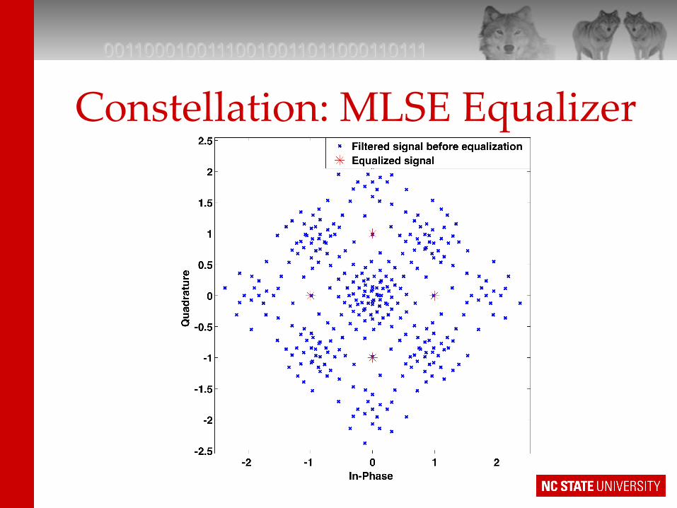
Constellation:  MLSE  Equalizer

00110001001110010011011000110111

Simulation:  Symbol  Error  Rate   •  SER  increases  with  M

•  Change  is  larger  for  Linear  Equalizer.  

•  So  does  DFE  and  MLSE.

  •  MLSE  is  the  optimum  

choice   •  relatively  low  SER,  and  

the  other   •  The  other  two  are  

suboptimum

[1] http://www.mathworks.com/help/comm/ug/equalization.html?refresh=true

M=8 M=16 M=32 Linear 0.357 0.592 0.824 DFE 0.091 0.136 0.532 MLSE 0.010 0.023 0.044

0.000 0.100 0.200 0.300 0.400 0.500 0.600 0.700 0.800 0.900

Sym

bol E

rror

Rat

e

Symbol Error Rate Comparision

00110001001110010011011000110111

•  The  runtime  for  LE  and  DFE  is  very  low:   •  around  0.07s  to  0.08s, •  Doesn’t  change  as  M  

increases.  

•  Runtime  for  MLSE  was  off  the  charts.  Literally! •  It  grows  exponentially  

as  M  increases. •  Takes  423  sec  at  M=32

[1] http://www.mathworks.com/help/comm/ug/equalization.html?refresh=true

M=8 M=16 M=32 Linear 0.070 0.079 0.073 DFE 0.074 0.083 0.075

0.060

0.065

0.070

0.075

0.080

0.085

Run

tim

e (s

econ

ds)

Equalization Time Comparision (Linear and DFE)

M=8 M=16 M=32 MLSE 2.020 22.319 422.884

0.000

50.000

100.000

150.000

200.000

250.000

300.000

350.000

400.000

450.000

Run

tim

e (s

econ

ds)

Equalization Time (MLSE)

Simulation:  Runtimes

00110001001110010011011000110111

Summary • MLSE  is  the  optimum  choice  from  the  respect  of  accuracy  with  relatively  high  complexity.

• While  LE  and  DFE  are  suboptimum  in  SER  but  take  shorter  runtime.  

• Unavoidable  tradeoff • There  newer  equalization  tools  like  Turbo  Equalizer.