factor markets - federal reserve bank of st. louis · importance of factor markets • determine...
TRANSCRIPT

Factor Markets
AP Economics | June 19, 2014 | Grant Black
Center for Entrepreneurship
and Economic Education
University of Missouri-St. Louis
Introduction
• Factors of production and factor markets
• Factor income
• Derived demand for factors of production
• Productivity theory and factor markets
– Marginal revenue product
– Marginal resource cost
– Profit maximization
Introduction
• Productivity theory and factor markets
– Effect of imperfect competition in product
markets
– Effect of imperfect competition in labor markets
– Monopsony
• Problems with productivity theory in factor
markets
• Government intervention in factor markets:
minimum wage

Factors of Production
• Any resource used to produce goods and services
– Labor
– Land and other natural resources
– Capital (physical and human)
• Factors of production earn income from the
ongoing selling of their services
• Factor markets = markets where factors of
production are traded
– Households are suppliers
– Firms are demanders
Importance of Factor Markets
• Determine prices of resources
• Allocate productive resources to producers
• Help ensure resources are used efficiently
Factor Income
• Sale of factors of production usually
generates largest share of most people’s
incomes
• Factor distribution of income = how total
income in the economy is divided among
labor, land, and capital
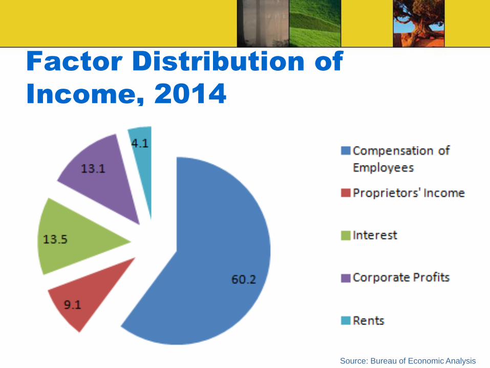
Factor Distribution of
Income, 2014
Source: Bureau of Economic Analysis
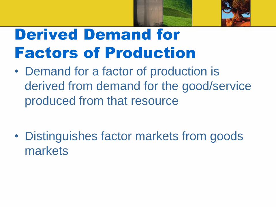
Derived Demand for
Factors of Production
• Demand for a factor of production is
derived from demand for the good/service
produced from that resource
• Distinguishes factor markets from goods
markets
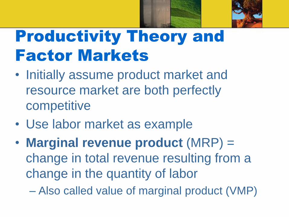
Productivity Theory and
Factor Markets
• Initially assume product market and
resource market are both perfectly
competitive
• Use labor market as example
• Marginal revenue product (MRP) =
change in total revenue resulting from a
change in the quantity of labor
– Also called value of marginal product (VMP)
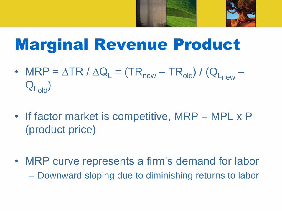
Marginal Revenue Product
• MRP = ∆TR / ∆QL = (TRnew – TRold) / (QLnew –
QLold)
• If factor market is competitive, MRP = MPL x P
(product price)
• MRP curve represents a firm’s demand for labor
– Downward sloping due to diminishing returns to labor
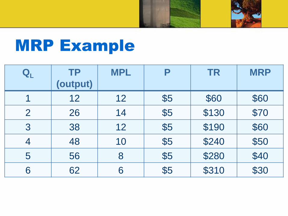
MRP Example
QL TP
(output)
MPL P TR MRP
1 12 12 $5 $60 $60
2 26 14 $5 $130 $70
3 38 12 $5 $190 $60
4 48 10 $5 $240 $50
5 56 8 $5 $280 $40
6 62 6 $5 $310 $30
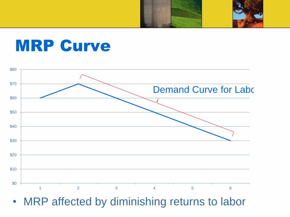
MRP Curve
• MRP affected by diminishing returns to labor
$0
$10
$20
$30
$40
$50
$60
$70
$80
1 2 3 4 5 6
Demand Curve for Labor
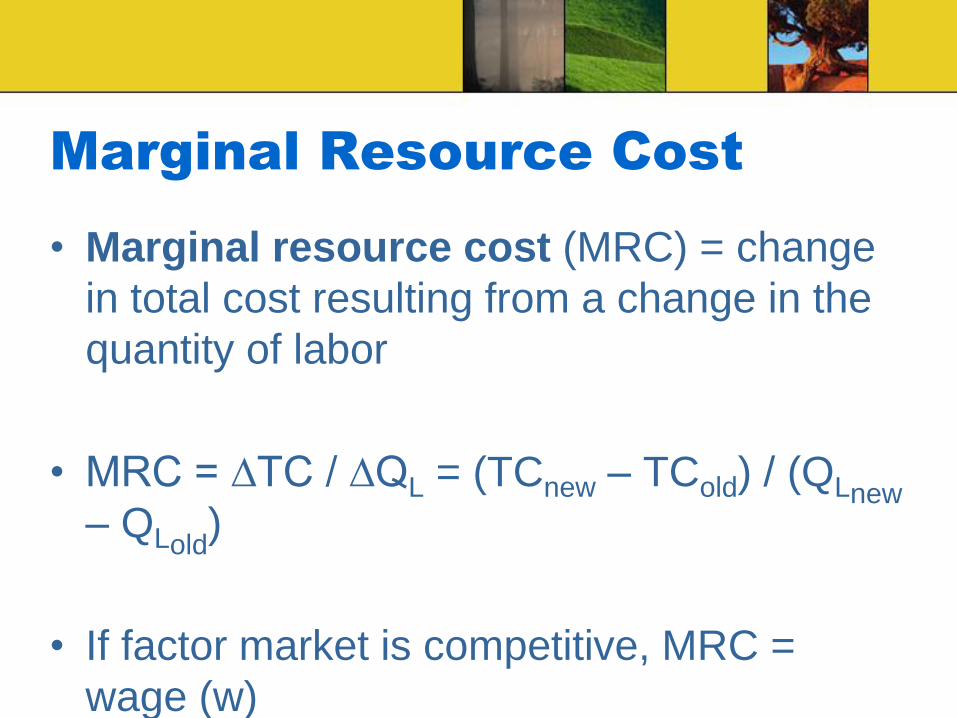
Marginal Resource Cost
• Marginal resource cost (MRC) = change
in total cost resulting from a change in the
quantity of labor
• MRC = ∆TC / ∆QL = (TCnew – TCold) / (QLnew
– QLold)
• If factor market is competitive, MRC =
wage (w)
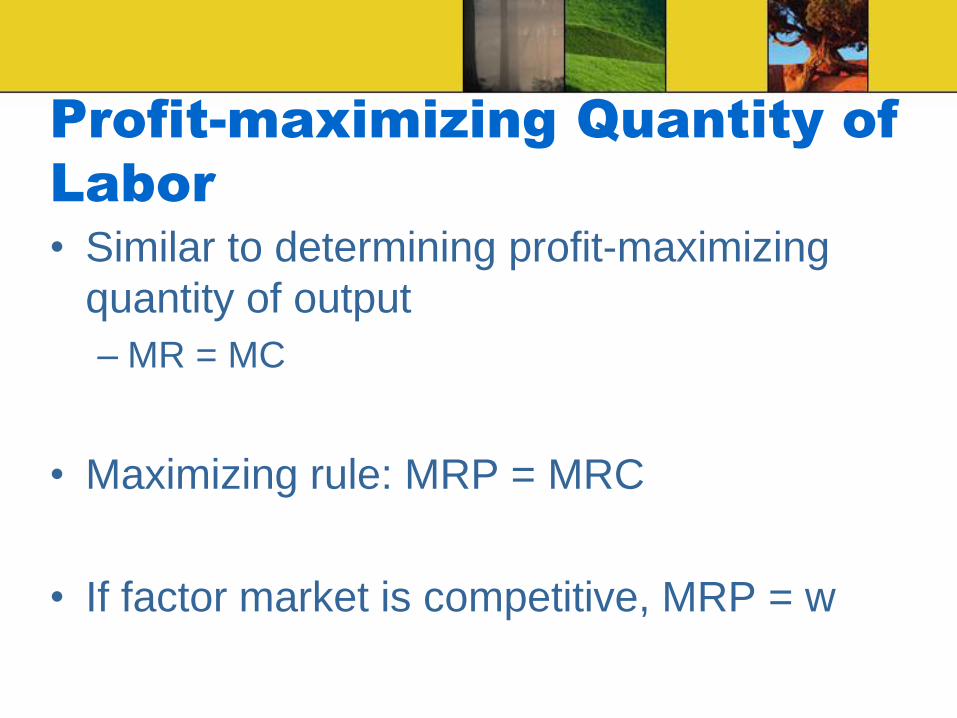
Profit-maximizing Quantity of
Labor
• Similar to determining profit-maximizing
quantity of output
– MR = MC
• Maximizing rule: MRP = MRC
• If factor market is competitive, MRP = w
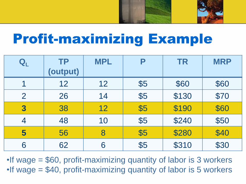
Profit-maximizing Example
QL TP
(output)
MPL P TR MRP
1 12 12 $5 $60 $60
2 26 14 $5 $130 $70
3 38 12 $5 $190 $60
4 48 10 $5 $240 $50
5 56 8 $5 $280 $40
6 62 6 $5 $310 $30
•If wage = $60, profit-maximizing quantity of labor is 3 workers
•If wage = $40, profit-maximizing quantity of labor is 5 workers
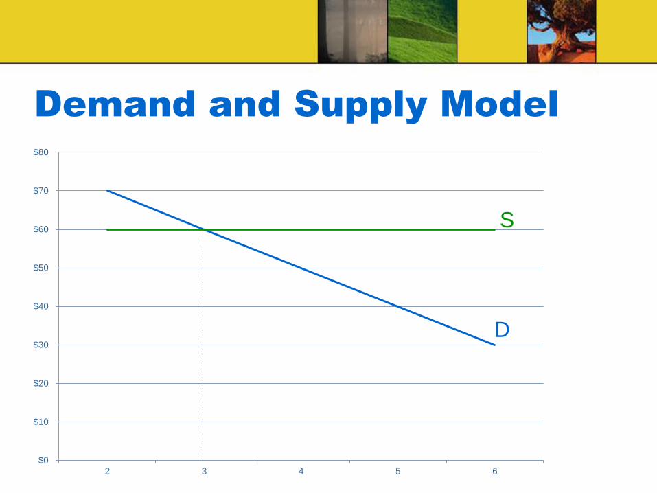
Demand and Supply Model
$0
$10
$20
$30
$40
$50
$60
$70
$80
2 3 4 5 6
D
S

$0
$10
$20
$30
$40
$50
$60
$70
$80
2 3 4 5 6
S
Demand and Supply Model
S’
D
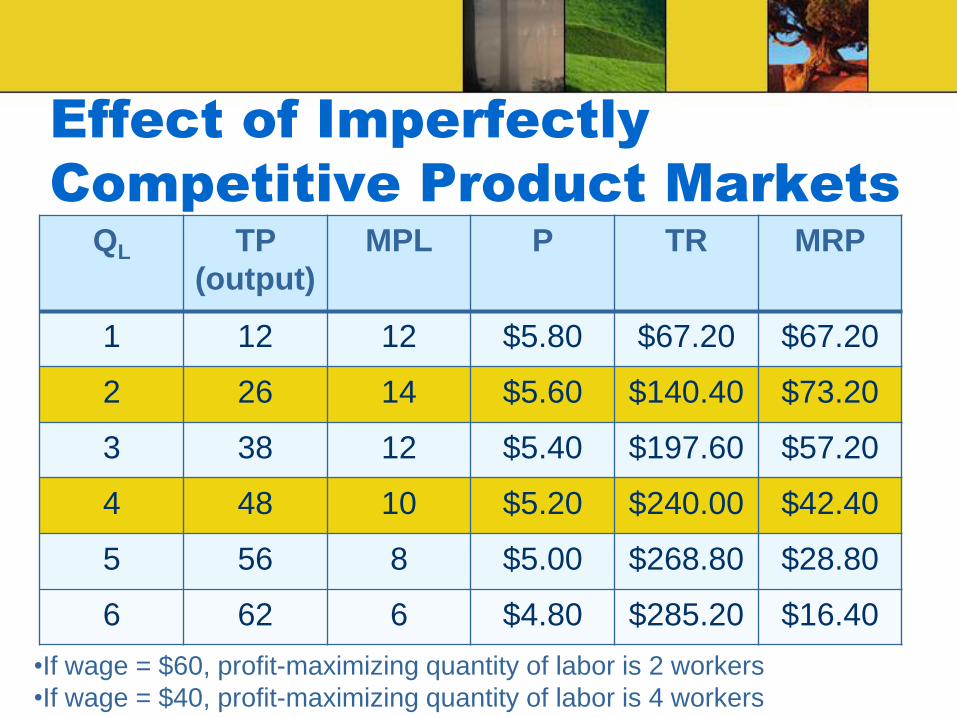
Effect of Imperfectly
Competitive Product Markets
QL TP
(output)
MPL P TR MRP
1 12 12 $5.80 $67.20 $67.20
2 26 14 $5.60 $140.40 $73.20
3 38 12 $5.40 $197.60 $57.20
4 48 10 $5.20 $240.00 $42.40
5 56 8 $5.00 $268.80 $28.80
6 62 6 $4.80 $285.20 $16.40
•If wage = $60, profit-maximizing quantity of labor is 2 workers
•If wage = $40, profit-maximizing quantity of labor is 4 workers
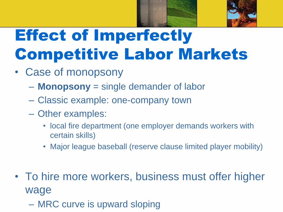
Effect of Imperfectly
Competitive Labor Markets
• Case of monopsony
– Monopsony = single demander of labor
– Classic example: one-company town
– Other examples:
• local fire department (one employer demands workers with
certain skills)
• Major league baseball (reserve clause limited player mobility)
• To hire more workers, business must offer higher
wage
– MRC curve is upward sloping
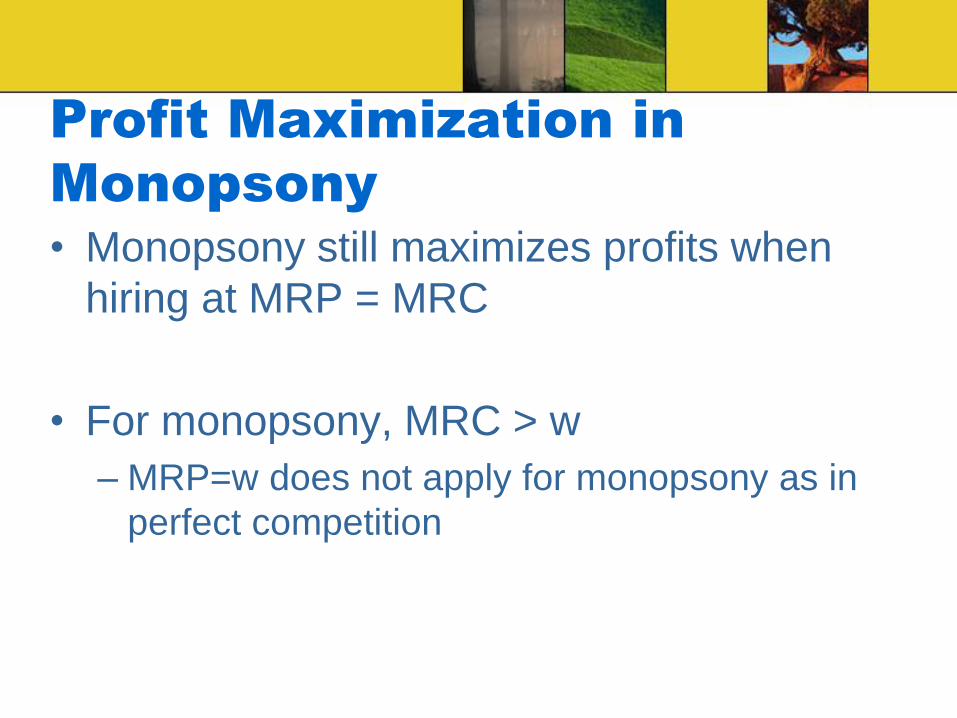
Profit Maximization in
Monopsony
• Monopsony still maximizes profits when
hiring at MRP = MRC
• For monopsony, MRC > w
– MRP=w does not apply for monopsony as in
perfect competition
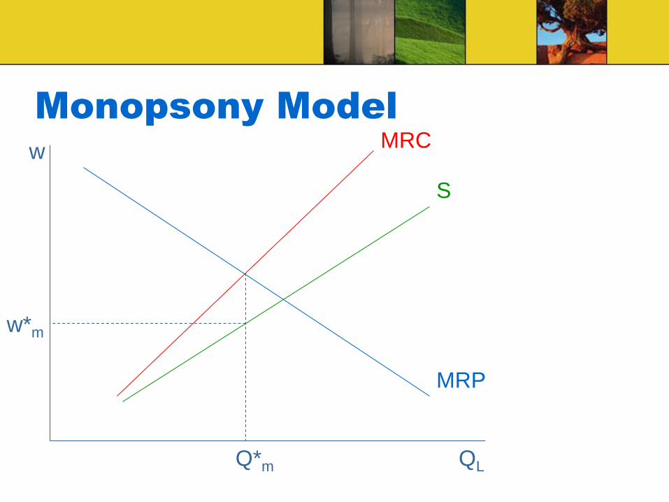
Monopsony Model
QL
w
Q*m
w*m
MRP
S
MRC
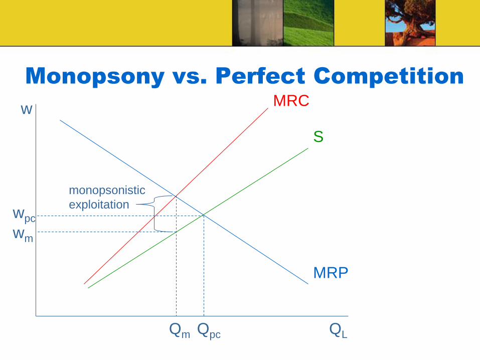
Monopsony vs. Perfect Competition
QL
w
Qm
wm
MRP
S
MRC
wpc
Qpc
monopsonistic
exploitation
Problems with Productivity
Theory in Factor Markets
• In real world, substantial differences exist
between prices of factors that likely have
similar MRP
– Wage gaps by gender and race
• In real world, some resources are not fully
employed and may receive prices higher
than their MRP or market-clearing levels

Median Weekly Earnings by
Gender and Race, 2014
White
Men
Women (all
races/ethnicities)
African
American (men
and women)
Hispanic
(men and
women)
$948 $754 $682 $651
*For those aged 25 and over
Source: Bureau of Labor Statistics
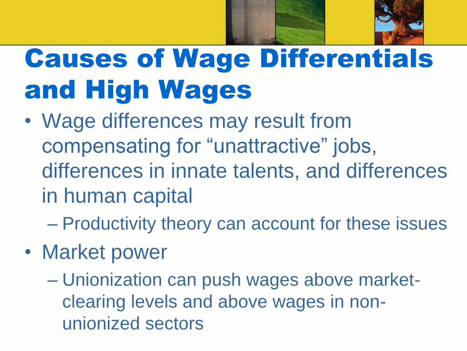
Causes of Wage Differentials
and High Wages
• Wage differences may result from
compensating for “unattractive” jobs,
differences in innate talents, and differences
in human capital
– Productivity theory can account for these issues
• Market power
– Unionization can push wages above market-
clearing levels and above wages in non-
unionized sectors
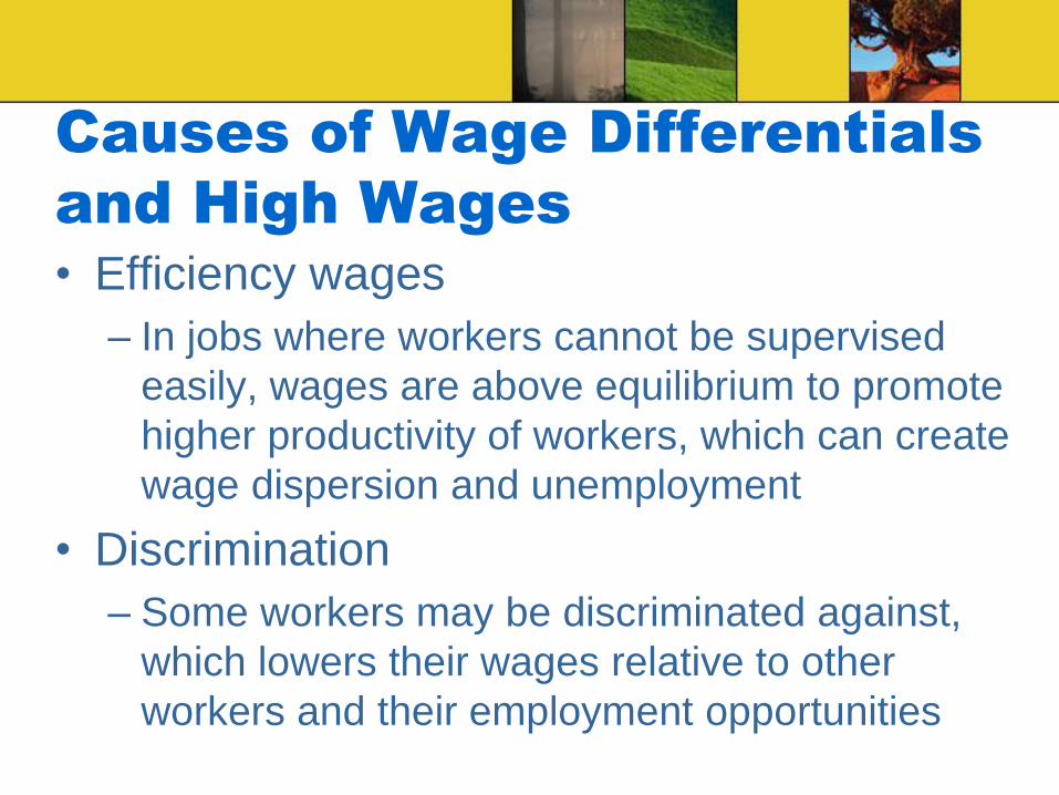
Causes of Wage Differentials
and High Wages
• Efficiency wages
– In jobs where workers cannot be supervised
easily, wages are above equilibrium to promote
higher productivity of workers, which can create
wage dispersion and unemployment
• Discrimination
– Some workers may be discriminated against,
which lowers their wages relative to other
workers and their employment opportunities
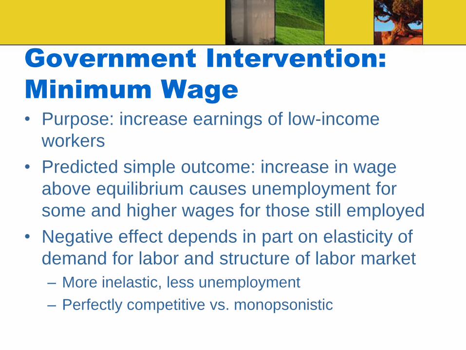
Government Intervention:
Minimum Wage
• Purpose: increase earnings of low-income
workers
• Predicted simple outcome: increase in wage
above equilibrium causes unemployment for
some and higher wages for those still employed
• Negative effect depends in part on elasticity of
demand for labor and structure of labor market
– More inelastic, less unemployment
– Perfectly competitive vs. monopsonistic
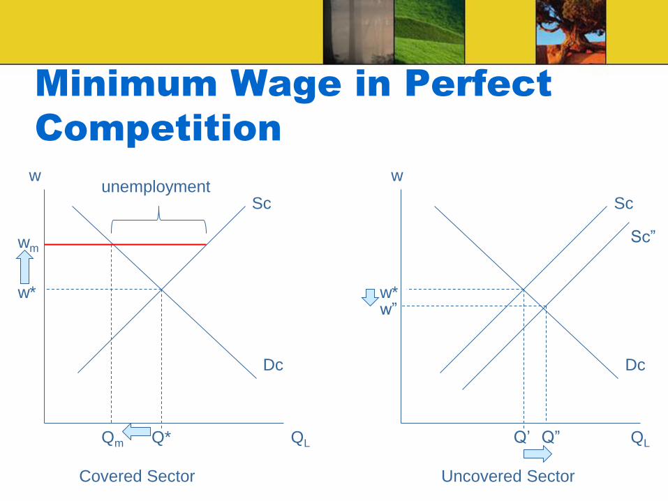
Minimum Wage in Perfect
Competition
Sc
Dc
w
QL
w*
Q*
wm
unemployment
Qm
Covered Sector
Sc
Dc
w
QL
w*
Q’ Q”
Uncovered Sector
Sc”
w”
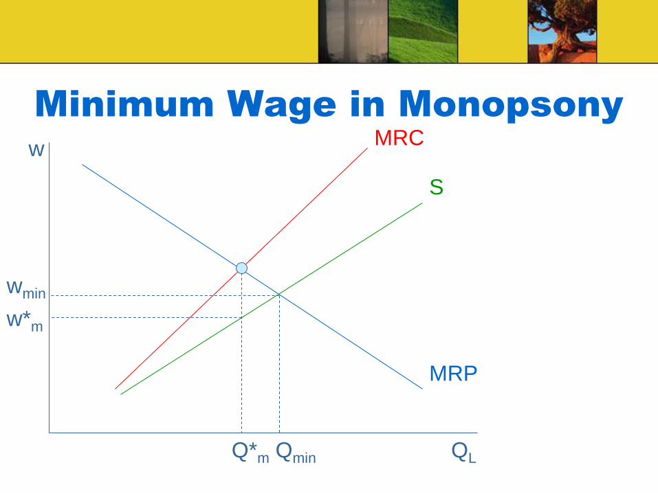
Minimum Wage in Monopsony
QL
w
Q*m
w*m
MRP
S
MRC
wmin
Qmin

Wrap Up
Questions?
Grant Black
Center for Entrepreneurship and Economic Education
University of Missouri-St. Louis
314-516-5248