古典Yang-Mills系における 　　　カラーグラス凝縮状態からの熱化過程

H.Iida, T.Kunihiro (Dept. of Phys., Kyoto Univ.), A.Ohnishi (YITP, Kyoto Univ.)

B.Müller (Duke Univ.), A.Schäfer (Regensburg Univ.), T.T.Takahashi (Gumma Nat. Col. of Tech.)

A.Yamamoto (RIKEN)

Thermal Quantum Field Theory and Their Applications 2012 @ YITP, 22 Aug., 2012

Contents

  Introduction   Early thermalization in Heavy-Ion Collision   Entropy production in quantum mechanics and classical dynamics

… Kolmogorov-Sinai Entropy & Husimi-Wehrl Entropy   Entropy production in Classical Yang-Mills dynamics

  Entropy production from Color-glass condensate initial condition

  Summary and conclusions

Introduction   Early thermalization: mystery of Heavy Ion Collision

PT and centrality dependence of π, p in Au+Au collision at \root s=130 A GeV, taken by the PHENIX and STAR collab.

(RHIC white paper & U.Heinz and P.Kolb, arXiv:hep-ph/0111075.)

τeq=0.6fm/c … early thermalization

Thermalization process in heavy ion collision is important.

cf) pQCD: τeq>2fm/c (K.Geiger 1992)

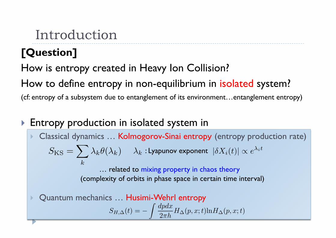
Introduction [Question] How is entropy created in Heavy Ion Collision? How to define entropy in non-equilibrium in isolated system? (cf: entropy of a subsystem due to entanglement of its environment…entanglement entropy)

  Entropy production in isolated system in   Classical dynamics … Kolmogorov-Sinai entropｙ (entropy production rate)

  Quantum mechanics … Husimi-Wehrl entropy

: Lyapunov exponent

… related to mixing property in chaos theory (complexity of orbits in phase space in certain time interval)

|�Xi(t)| � e�it

・Distribution function in q.m. …Wigner function??:

・Husimi function:

- Husimi-Wehrl entropy

… not always positive

� 0(�: smearing parameter)

Can we construct a quantity like H function in quantum mechanics?

Husimi-Wehrl entropy

… H is obtained by smearing W with minimum uncertainty in phase space

Relation bw KS and HW entropy

dSH,�

dt� � (t��) (t� ��1)

Important observation: Coarse grained quantum mechanical (HW) entropy growth rate agrees with KS entropy.

●

●

●

・The growth rate of the Husimi-Wehrl entropy is given by the K-S entropy (positive Lyapunov exponent) in the classical dynamics! ・Unstable modes in the classical dynamics plays the essential role for entropy production at quantum level.　 → may account for entropy production in quantum level in HI collisions at RHIC.

Ref.) T.Kunihiro,B.Mueller, A.Ohnishi, A.Schaefer, PTP121 (2009)

…slightly different from at initial time, respectively

s

Entropy production in classical Yang-Mills dynamics

  Focusing on entropy production through the chaotic behavior in Classical Yang-Mills system.

|�Xi(t)| � e�it… related to chaoticity

Entropy production rate (Kolmogolov-Sinai entropy)

s Distance between two trajectories in phase space

Two quantities

T.Kunihiro, B.Mueller, A.Ohnishi, A.Schaefere, T.T.Takahashi and A.Yamamoto, PRD82, 114015(2010).

  Entropy production & early thermalization is investigated in CYM with random initial condition

Entropy production in classical Yang-Mills dynamics

Time evolution of δX for several initial energy density

Time evolution of Lyapunov exponent

T.Kunihiro, B.Mueller, A.Ohnishi, A.Schaefere, T.T.Takahashi and A.Yamamoto, PRD82, 114015(2010).

In this study

  Study of early thermalization in heavy-ion collisions using classical Yang-Mills eq. with CGC-like initial conditions in non-expanding plasma

(initial gauge field has some spatial correlations)

  We focus on the chaotic behavior of the systems: distance between two trajectories with slightly different initial conditions & Lyapunov exp.

Color-glass condensate

  High energy collision… high gluon density → gluons are coherent field rather than particles First approximation: classical treatment

  Initial condition: color-glass condensate (CGC) (L.McLerran and R.Venugopalan 1994; T.Lappi and L.McLerran 2006, …)

Classical Yang-Mills calculation with CGC initial condition … appropriate for the study of thermalization process

  Instability … served as a possible mechanism of early thermalization (Weibel instability… S.Mrowczynski, Nielsen-Olesen instability… Fujii, Itakura; Fujii, Itakura, Iwazaki)

1.  Modulated  initial  condition

Fluctuation (noise)

Magnetic field from spatial modulation (neglecting noise)

x

zy

(+ fluctuation)

magnetic field

Results: modulated init. cond.

  Time evolution of gauge fields

Red arrow:

Green arrow:

Ai

Ei

“Instability” (chaotic behavior?) seems to occur for large t

SU(2), 43

(time evolution of two trajectories from very similar init. cond.)

…slightly different from at initial time, respectively

|�Xi(t)| � e�itcf) Lyapunov exponent

:governed by maximum Lyapunov exp.

Distance between two trajectories

-10

-9

-8

-7

-6

-5

-4

0 50 100 150 200 250 300

log(

DFF

) or l

og(D

EE)

t

DFF and DEE

DFFDEE

-10

-9

-8

-7

-6

-5

-4

0 50 100 150 200 250 300

log(

DFF

) or l

og(D

EE)

t

DFF and DEE

DFFDEE-12

-11

-10

-9

-8

-7

-6

-5

-4

0 50 100 150 200 250 300

log(

DFF

) or l

og(D

EE)

t

DFF and DEE

DFFDEE

Results: time dep. of distance

only fluctuation only modulation

modulation + fluctuation

・Modulation only … No chaotic behavior ・Modulation + (tiny) fluctuation…chaotic behavior occurs

-10

-9

-8

-7

-6

-5

0 20 40 60 80 100 120 140 160

log(

DFF

)

t

DFF

only fluctuationw=0.0001w=0.0004w=0.0008w=0.0016

Distances for various initial fluctuation

Onset time of increase of D depends on the ratio of fluctuation to background modulation field

large fluctuation

  Time evolution of difference between two trajectories:

  We can formally solve the equation for finite :

  Using Trotter formula, U is written as

  By diagonalization, ILE is obtained:

(Hxx)ij = �2H/�xi�xj

Hessian H

Intermediate Lyapunov exponent

We set

0

0.02

0.04

0.06

0.08

0.1

0.12

0.14

0 50 100 150 200

Intermediate Lyapunov exponent

t=50t=70

t=100t=150t=200

Results: Intermediate Lyapunov exp.

・Distribution of Lyapunov exp. is stable at large t, and then, significant portion of Lyapunov exponents  keeps positive in a robust way → chaotic

0

0.05

0.1

0.15

0.2

0.25

0.3

0.35

0.4

0.45

0.5

0 50 100 150 200

Intermediate Lyapunov exponent

t=0t=5

t=40t=50

・Instability spreads to many modes in the very early stage.

-10

-9

-8

-7

-6

-5

-4

0 50 100 150 200 250 300

log(

DFF

) or l

og(D

EE)

t

DFF and DEE

DFFDEE

# of ILE = V*(Nc2-1)*3*2

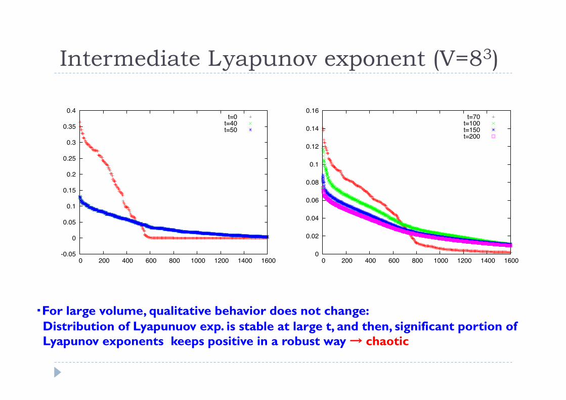
Intermediate Lyapunov exponent (V=83)

・For large volume, qualitative behavior does not change: Distribution of Lyapunuov exp. is stable at large t, and then, significant portion of Lyapunov exponents  keeps positive in a robust way → chaotic

0

0.02

0.04

0.06

0.08

0.1

0.12

0.14

0.16

0 200 400 600 800 1000 1200 1400 1600

t=70t=100t=150t=200

-0.05

0

0.05

0.1

0.15

0.2

0.25

0.3

0.35

0.4

0 200 400 600 800 1000 1200 1400 1600

t=0t=40t=50

2.  Constant  A  initial  condition

Aai (�r) = �a

i (�r) + (�a2�xi + �a3�yi)

�B

g

Eai (�r) = 0

Magnetic field (neglecting noise)

Others: zero

x

zy

(+ fluctuation)

Ref.) J.Berges, S.Scheffler, S.Schlichting and D.Sexty

Results: constant A init. cond.

Red arrow:

Green arrow:

Ai

Ei

“Instability” (chaotic behavior?) seems to occur for large t.

•  Time evolution of gauge fields

-10

-9

-8

-7

-6

-5

-4

0 50 100 150 200 250 300

log(

DFF

) or l

og(D

EE)

t

DFF and DEE

DFFDEE

Results: time dep. of distance   (2) Constant magnetic field

D becomes large (with oscillation)

・Modulation + (tiny) fluctuation…chaotic behavior occurs also in the initial condition

0

0.05

0.1

0.15

0.2

0.25

0 50 100 150 200In

term

edia

te L

yapu

nov

expo

nent

t=50t=70

t=100t=150t=200

ILE for Constant A

-0.05

0

0.05

0.1

0.15

0.2

0.25

0.3

0.35

0.4

0 50 100 150 200

Inte

rmed

iate

Lya

puno

v ex

pone

nt

t=0t=5

t=40t=50

-10

-9

-8

-7

-6

-5

-4

0 50 100 150 200 250 300

log(

DFF

) or l

og(D

EE)

t

DFF and DEE

DFFDEE

・Although the distribution of ILE in initial stage is different from that in modulated initial condition (MIC), the distribution in later stage is similar to that in MIC.

ILE for Constant A (V=83)

0

0.05

0.1

0.15

0.2

0.25

0 200 400 600 800 1000 1200 1400 1600

t=70t=100t=150

0

0.05

0.1

0.15

0.2

0.25

0.3

0.35

0.4

0 200 400 600 800 1000 1200 1400 1600

t=0t=40t=50

・For large volume, qualitative behavior does not change: Distribution of Lyapunuov exp. is stable at large t, and then, significant portion of Lyapunov exponents  keeps positive in a robust way → chaotic

Summary and conclusions

•  Background  magne.c  field  +  (.ny)  fluctua.on                                                                                                                                              →  chao.c  behavior  

•  Behavior  of  intermediate  Lyapunov  exponent:  Distribu.on  of  Lyapunov  exponent  seems  to  be  stable    at  large  t,  and  then,  significant  por.on  of  Lyapunov  exponents  keeps  posi.ve  in  a  robust  way.  

・Entropy production proceeds already in the CYM evolution. ・The entropy production in CYM may serve as a possible mechanism of early thermalization. ・Initial fluctuation has important role for the mechanism.

Various kind of distance

Various kind of distances

・Different definitions give different slopes ・DEE & DFF are almost the same