munich personal repec archive - mpra.ub.uni-muenchen.de · munich personal repec archive linepack...
TRANSCRIPT

MPRAMunich Personal RePEc Archive
Linepack storage valuation under priceuncertainty
Øystein Arvesen and Vegard Medbø and Stein-Erik Fleten
and Asgeir Tomasgard and Sjur Westgaard
Norwegian University of Science and Technology (NTNU)
7 November 2012
Online at https://mpra.ub.uni-muenchen.de/43270/MPRA Paper No. 43270, posted 14 December 2012 14:03 UTC

Linepack storage valuation under price uncertainty
Ø. Arvesen, V. Medbø, S.-E. Fleten∗, A. Tomasgard, S. Westgaard
Norwegian University of Science and Technology, NO–7491 Trondheim, Norway
Abstract
Natural gas flows in pipelines as a consequence of the pressure difference at
the inlet and outlet. Adjusting these pressures makes it possible to inject
natural gas at one rate and withdraw at a different rate, hence using the
pipeline as storage as well as transport. We study the value of using the so
called pipeline linepack as a short-term gas storage and how this function-
ality may offset the discrepancy between the low flexibility in take-or-pay
contracts and the high inherent flexibility of a gas fired power plant. To
value the storage option, we consider a cycling power plant facing volatile
power prices while purchasing gas on a take-or-pay contract. We estimate a
Markov regime-switching model for power prices and a mean reverting jump
diffusion model for gas prices. Applying Least Squares Monte Carlo simu-
lation to the operation of the power plant, we find that the storage option
indeed has significant value for the plant, enabling it to better exploit the
sometimes extreme price fluctuations. Finally, we show how power price
∗Corresponding author. Tel.: +47 73591296; fax: +47 73591045Email addresses: [email protected] (Ø. Arvesen),
[email protected] (V. Medbø), [email protected] (S.-E.Fleten), [email protected] (A. Tomasgard),[email protected] (S. Westgaard)
Preprint submitted to Energy November 7, 2012

volatility and jump frequency are the main value drivers, and that the size of
the storage increases the value up to a point where no additional flexibility
is used.
Keywords: Linepack, Gas storage valuation, Regime-switching models,
Natural gas prices, Electricity prices, Power plant
1. Introduction
Pipelines are the largest infrastructure investment in the natural gas value
chain, accounting for 80 percent of midstream investments [1]. To provide
both security of supply as well as a high standard of safety, the pressure
of the pipelines must be kept within a certain range. By controlling the
pressures, the stored gas in the pipeline (linepack) can increase or decrease
as the withdrawal and injection rates differ from each other. We show that
making part of the linepack available for the market as a storage volume
can be a viable option to increase the flexibility of the energy system. Such
increased flexibility is highly attractive in light of the intermittency of much
of the future electricity generation sources [2].
We take the perspective of a German gas-fired power plant in order to
analyse the value of using e.g. the North Sea pipeline system as a short term
storage volume. This connection is not identified as congested [3], and has
a reliability of “virtually 100%” [4]. The participant with the highest need
for flexibility in its gas flows should be the one with highest willingness to
pay for the storage. Arguably, a gas-fired power plant facing uncertainty in
both electricity and gas prices can be such a participant. In Europe, the
plant will often be committed to a long-term take-or-pay (TOP) contract,
2

forcing the plant to buy a certain volume of gas per year. The high degree
of uncertainty in prices with combined with a low degree of flexibility in the
TOP contract makes additional flexibility valuable. Modern gas-fired power
plants are able to ramp production up and down on short time notice. As
most industrial processes that use gas as a primary input do not have the
same degree of operational flexibility nor the same degree of participation in
the gas spot market, we view a cycling gas-fired power plant as the agent
with the highest incentive to pay for storage opportunities. Approximately
36 percent of the natural gas consumption in OECD Europe is consumed by
power plants [5], implying that the sector should be vital in the demand for
gas storage capacity. We estimate the additional value created by using the
linepack to vary the power plant’s output rate according to swings in the
prices of power and natural gas, without violating the TOP contract.
Conventional storage capacity, consisting of depleted oil and gas reser-
voirs, aquifers, salt mines and LNG storage plants, are in most cases con-
strained by their geographical location and a rather low inflow and with-
drawal rate. Furthermore, LNG plants have high storage costs since the gas
needs to be cooled [6]. The pipeline exit point is usually situated at a major
market hub. Considering the linepack as a separate storage volume placed
at the receiving terminal, the high flexibility makes it a potentially valuable
tool for short-term balancing of natural gas supply and demand.
We focus only on the value of the line pack, and ignore cost issues re-
lated to fuel consumption in compressor stations, or a possible loss of supply
reliability, or pipeline capacity. That said, we note that linepack is highly
flexible as long as it is within upper and lower bound based on the technical
3

characteristics of the pipeline.
Midthun et al. [7] value the linepack as a natural gas storage facility,
taking the perspective of a natural gas producer. They optimise the value
of the gas sales for the producer both with and without the linepack, and
quantify the size of a pipeline’s possible linepack. Chaudry et al. [8] include
linepack in optimisation of the GB gas and electricity network. Our paper
shifts the focus on the value of linepack storage from that of a producer to
that of a consumer of natural gas.
Keyaerts et al. [9] call for a change of the regulatory framework for natu-
ral gas pipeline capacity allocation in Europe, taking linepack into account.
They point out value and cost components of linepack flexibility and identify
the trade-off in its use as storage flexibility and transportation facility.
Storage valuation literature focus either on best practice power price sim-
ulation, gas price simulation or on valuing a general storage volume in the
perspective of a commodity arbitrageur. Boogert and de Jong [10] apply the
Least Squares Monte Carlo algorithm, developed by Longstaff and Schwartz
[11], to value a natural gas storage contract. They show that the size of the
effective storage volume as well as injection and withdrawal rates are the
most important value-determinants. Lai et al. [12] value the option to store
natural gas in the form of LNG using a heuristic that incorporates natural
gas prices, LNG shipping models and inventory control. Bjerksund et al. [13]
show that an advanced price process is of greater importance than a an ad-
vanced optimisation model, when valuing gas storage. Valuation of storage
in connection with CO2 capture plants is considered by [14, 15]. Finally, [16]
value biomass storage in the context of a biomass supply chain.
4
Authors including de Jong [17], Janczura and Weron [18] and Schneider
[19] agree that the power price exhibits mean reversion and spikes. Abadie
and Chamorro [20] show that natural gas spot prices exhibit mean reversion.
Secomandi [21] analyses the pricing of pipeline capacity based on the trading
value of the gas, modeled as a mean reverting process. As an alternative, a
nonstationary process such as geometric Brownian motion can be used for
gas [22] or electricity prices [23], however, these are more suitable for a) long
planning horizons (decades), or b) when analytical solutions are preferred
[24].
The main contribution of this paper is the quantification of the value of
linepack as storage of natural gas, from a gas consumer point of view. For
power systems with increased use of intermittent renewable sources, pointing
to ignored but potentially useful energy storage options is of high value. In
addition, the Markov regime-switching model for electricity prices, incorpo-
rating spikes, mean reversion and possible negative prices, is state of the art.
Finally, we introduce a gas price model with a mean level that depends on
electricity prices, so that a realistic long-term relationship between prices of
electricity and natural gas prevails.
The article is structured as follows: In Section 2 we describe the data used
and estimate models that capture the joint dynamics of natural gas and power
prices. We estimate a Markov regime-switching model with independent
spikes for the power price, and a mean reverting jump diffusion model for the
gas price, where the mean level is dependent on the power price. Simulating
the two price series simultaneously, we essentially model the power plant’s
5

dirty spread1. In Section 3, we apply a real option approach and incorporate
the price models in a Least Squares Monte Carlo algorithm to value the
opportunity of storage. Our analysis is confined to valuing the storage option
separately, disregarding the power plant’s intrinsic value. We show numerical
examples to illustrate how parameters such as storage capacity and price
volatility affect the storage value in Section 4. In Section 5 we conclude.
2. Model description
To be able to value a gas storage facility, we need to accurately model
the power price and the gas price. The models must capture the seasonal
patterns, its stochastic behaviour and the way gas and power prices move
together. We first model the power price, and then use it as an explana-
tory variable in the gas price model. These two models will be used in the
simulation based valuation algorithm in Section 3.
2.1. Power price model
The data set used for power prices consists of hourly data from the EPEX
commodity exchange in Germany, from 2011-01-03 until 2011-10-23; a total
of 7056 data points. In general, the prices exhibit a strong degree of hour-of-
day effects and weekday effects. In addition, sudden spikes are clearly visible
in Figure 1, but they seem to disappear just as soon as they arrive. There
also seems to be a certain degree of clustering of spikes.
1The dirty spread is the spread between the power price and the price of the gas needed
to produce the power before subtracting the CO2 price.
6

-60
-40
-20
0
20
40
60
80
100
120
140
jan. 11 feb. 11 mar. 11 apr. 11 mai. 11 jun. 11 jul. 11 aug. 11 aug. 11 sep. 11
Figure 1: The time series of hourly power prices at EPEX.
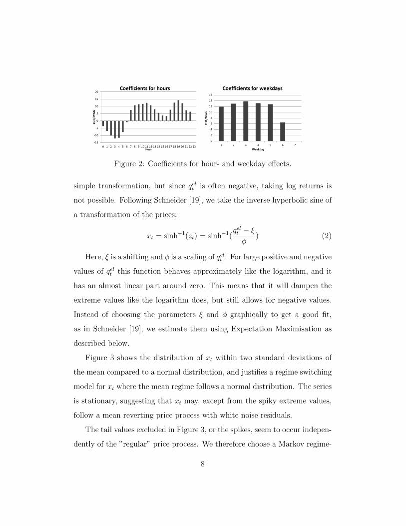
To analyse the stochastic part of the data, we first filter out the determin-
istic effects by simple dummy variables for hours and weekdays and store the
residuals. The typical daily and weekly pattern of power prices are apparent
in the dummy coefficients given in Figure 2, all of which are significant at
the 5% level. In mathematical terms:
Selt = µel0 +6∑i=1
δweekdayi θeli +23∑j=1
δhourj γelj + qelt (1)
where Selt is the electricity price, µel0 is a constant, θel are coefficients for
weekdays and γel are coefficients for hours. The δs are binary variables that
indicate whether a price observation is from a certain weekday or hour. Note
that one day and one hour is left out of the regression to avoid multicollinear-
ity.
After filtering out the deterministic effects, we are left with what we
will denote the stochastic component qelt . It has several spikes, and seems
to be mean reverting. We wish to dampen the extreme values through a
7
-15
-10
-5
0
5
10
15
20
0 1 2 3 4 5 6 7 8 9 10 11 12 13 14 15 16 17 18 19 20 21 22 23
EUR
/MW
h
Hour
Coefficients for hours
0
2
4
6
8
10
12
14
16
1 2 3 4 5 6 7
EUR
/MW
h
Weekday
Coefficients for weekdays
Figure 2: Coefficients for hour- and weekday effects.
simple transformation, but since qelt is often negative, taking log returns is
not possible. Following Schneider [19], we take the inverse hyperbolic sine of
a transformation of the prices:
xt = sinh−1(zt) = sinh−1(qelt − ξφ
) (2)
Here, ξ is a shifting and φ is a scaling of qelt . For large positive and negative
values of qelt this function behaves approximately like the logarithm, and it
has an almost linear part around zero. This means that it will dampen the
extreme values like the logarithm does, but still allows for negative values.
Instead of choosing the parameters ξ and φ graphically to get a good fit,
as in Schneider [19], we estimate them using Expectation Maximisation as
described below.
Figure 3 shows the distribution of xt within two standard deviations of
the mean compared to a normal distribution, and justifies a regime switching
model for xt where the mean regime follows a normal distribution. The series
is stationary, suggesting that xt may, except from the spiky extreme values,
follow a mean reverting price process with white noise residuals.
The tail values excluded in Figure 3, or the spikes, seem to occur indepen-
dently of the ”regular” price process. We therefore choose a Markov regime-
8

0
0,002
0,004
0,006
0,008
0,01
0,012
0,014
-1,6 -1,4 -1,2 -1 -0,8 -0,6 -0,4 -0,2 0 0,2 0,4 0,6 0,8 1 1,2 1,4 1,6
Figure 3: The empirical distribution of the capped prices compared to a
normal distribution.
switching (MRS) model with independent spikes, due to de Jong [17]. The
xt from eq. (2) follow a mean reverting process in one regime, and switches
to either a high-spike or a low-spike regime. The independence of regimes
means that if the price at t− 1 was generated by the low-spike regime, and
at t it is generated by the mean reverting regime, the price in time t will not
be influenced by how low it was in the previous period. What regime the
process is actually in is not observable, but we assume that the switching
between regimes is governed by a Markov transition matrix, Π. Recall that
xt = sinh−1(zt) = sinh−1(qelt −ξφ
), to handle negative prices. This renders the
model:
xMt = xMt−1 + αel(µel − xMt−1) + σelMεelt , εelt ∼ N(0, 1) (3)
xHt = µel +
nel,Ht∑i=1
Zel,Ht , nel,Ht ∼ POI(λelH), Zel,H
t ∼ N(µelH , σelH) (4)
9

xLt = µel +
nel,Lt∑i=1
Zel,Lt , nel,Lt ∼ POI(λelL), ZL
t ∼ N(µelL , σelL ) (5)
Π =
1− pMH − pML pHM pLM
pMH 1− pHM 0
pML 0 1− pLM
(6)
where entry pi,j in Π represents the probability of going from state j at
time t, to state i at time t + 1, (i, j) ∈ {1, 2, 3} and 1, 2 and 3 representing
regimes M,H and L respectively. As can be seen from the Markov transition
matrix, it is assumed that a transition from either a high spike to a low, or
the opposite, is impossible. The average xt is denoted µel and the speed
of mean reversion back to this level is αel, while the standard deviation of
residual variation is σelM . Note that the xts in the high spike regimes consist
of nel,Ht jumps, where each jump is normally distributed with mean µelH and
standard deviation σelH . The number of jumps is assumed to follow a poisson
process with rate parameter λelH , and correspondingly in the low spike regime.
The parameters above are estimated via the Expectation Maximisation (EM)
algorithm, largely following the original approach in Hamilton [25]. As the
spike regimes are independent of the mean reverting regime, the expected
price in the latter regime at time t is cumbersome to calculate. This is
because we can not observe how many of the previous observations that are
created by spike regimes, so all possible paths between times 0 and t should
be considered, a significant computational burden. To save computational
effort, we adopt the improvements proposed by Janczura and Weron [18] and
10

Table 1: Table of estimated parameters.
MRS model
Regime 1 2 3
αel 0.036
φ 7.599
ξ 38.460
µel -0.038 0.311 -0.373
σel 0.210 0.010 0.026
λel 1.842 - 1.899
pMH 0.009
pHM 0.129
pML 0.044
pLM 0.409
recursively approximate the expected price using the equation
E[xMt−1|xt−1] = ζ1,t|txt + (1− ζ1,t|t){αel · µel + (1− αel)E[xMt−2|xt−2]} (7)
Here, ζ1,t|s is the conditional probability of being in regime 1(= M) at time
t given the information available at time s ≤ t (see [18] for details). The
results of the estimation is displayed in Table 1.
This model was compared to a similar model with dependent spikes, sev-
eral GARCH-specifications and a parameter-switching model (Janczura and
Weron [18]), and outperformed all in terms of likelihood. Table 2 shows the
average descriptive statistics of 5000 simulations. Our valuation method is
based on Monte Carlo simulation, and the most important trait of our model
11

Table 2: Comparison of descriptive statistics from simulation with the actual values.
Actual Simulation
Mean 37.38 37.80
Standard Deviation 8.26 8.47
Skewness -1.22 -0.24
Kurtosis 8.79 9.01
is that the deterministic and stochastic patterns replicate the observed prices
well. We conclude that the MRS-model captures the dynamics in hourly
power prices well enough for our purposes, and that we will continue using
it in the valuation.
2.2. Gas price model
In modelling the gas price, we have used daily data for natural gas day-
ahead prices both in the German and the UK market. Although our mod-
elling is performed on the German market, we have used prices from UK’s
National Balancing Point as this time series has a history back to 1996. Net-
Connect Germany (NCG), Germany’s most liquid gas market, only has data
from 2007 onwards. Due to physical connections, gas prices in Northern Eu-
rope are closely integrated, and the NCG and NBP prices usually move in
tandem. To be sure that this is correct, we estimated the following model:
SNBPt = β0 + β1SNCGt + εNBPt (8)
where β0 is the difference in price between NBP and NCG and β1 is the
factor explaining how much of the NBP price that can be explained by the
12

price level of the NCG price. The results show that the coefficient β1 is
not significantly different from one on the 1% level, and that the NBP price
is on average 0.51 EUR/MWh higher than the NCG price. We will in the
following assume that the relationship SNBP = SNCG − 0.51 holds for all
points in time. Analysing the NBP price series in Figure 4, we first note that
there seems to be some trend, or price inflation, in the gas price. We can
also observe higher prices during winter and lower prices during summer.
As can be seen in Figure 4, the natural gas price exhibits mean reversion
and spikes that seem to arrive at random. Supply and demand imbalances
can cause the price to spike up or down, and return to the mean level during
the following days.
1
2
4
8
16
32
64
128
256
June-00 June-01 June-02 June-03 June-04 June-05 June-06 June-07 June-08 June-09 June-10 June-11
Phelix day base NBP
Figure 4: The NBP day-ahead gas price seems to fluctuate along with the
Phelix day-ahead power price. Note the occurrence of spikes in the NBP
price. Price axis in log scale.
We also note that the gas price moves along with the price of electric
13

power (see Figure 4).2 For the valuation of our gas storage, it is important
that we incorporate the covariation in the gas and power prices, ensuring that
the gas price does not move unrealistically high or low when compared to
the power price, as market forces likely would take effect and drive the prices
back to a long-term equilibrium. A price disequilibrium should result in gas-
fired power plants either ramping up or scaling down activity, and thereby
providing a counteractive force on the gap between gas and electricity prices.
We propose a process for the natural gas price, taking into account both the
spikes, mean reversion and the price level of electricity. Here, the mean level
for the gas price Sgt is µgt = E[Sgt |Selt ], where Selt is the electricity price. In
contrast to the power price, the gas price reverts more slowly from spikes,
i.e., they are not independent. Two spike functions are therefore added to
the price process with Poisson arrival rates λgH and λgL for the high and the
low spike process:
∆Sgt = αg(µgt − Sgt−1) +
ng,Ht∑i=1
Zg,Ht +
ng,Lt∑j=1
Zg,Lt + σgµgt ε
gt , εgt ∼ N(0, 1) (9)
µgt = µg0 + κSelt +11∑k=1
δmonthk θgk (10)
Here Sgt and Selt are the prices of gas and power at time t, µgt is the
2One would expect that in situations of cold weather, both electricity and gas demand
is high, and gas might be used as the marginal source of electricity. In such a situation,
one should expect a strong relationship between gas and electricity prices. In other market
conditions where demand is lower, one would expect prices of natural gas and electricity
to be less dependent on each other.
14

expected gas price and αg is the mean reversion rate. The expected gas
price consists of µg0, a constant, the influence of the power price κSelt and
the seasonal effect θgk if the binary variable δmonthk is one for month k. The
spike terms in eq. (9) are constructed exactly like in the power price model of
equations (4) and (5). Finally, the residual εgt is assumed standard normally
distributed and σg is a volatility parameter.
We thus allow the gas price to fluctuate as a mean reverting process
with spikes, but we set the mean level to be dependent on the level of the
electricity price. This is consistent with the results of de Jong and Schneider
[26]. We allow for high and low spikes, and we also allow for seasonal effects in
the gas price that are not explained by the seasonality of the power price. If
these seasonal variation parameters θgk are found to be statistically significant
(which we find that most of them are), the seasonal patterns in natural gas
differ from those of electricity.
This model is estimated in two steps: we first estimate the relationship
between the gas price and the electricity price, and in the second step we
estimate the mean reversion in the residuals qgt that is not explained by the
power price. The residual qgt is defined as:
qgt = Sgt − µgt (11)
where µgt is the expected mean level for the gas price. The first step is a
regression of the gas price on the power price and seasonal dummy variables
to find µgt , according to
Sgt = µg0 + κSelt +11∑k=1
δmonthk θgk + qgt (12)
15

Here we find the long-term relationship between the gas price and the
power price by determining µg0, κ and the different θgk. But as we wish to
model daily gas prices and hourly power prices for the valuation in Section 3,
we need to convert hourly power prices to a daily average given as Selt in
eq. (12). This was done by weighing 24 hourly power prices with the load
curves in Germany3. Also, this average day price is affected by price spikes
that seem to occur independently of the gas price—we therefore use the
arithmetic average of one week as Selt .
We now have an estimate of the expected gas price, E[Sgt |Selt ] = µgt , as
a function of the power price and the time of year, defined by the monthly
effects. The results are given in Table 3, with seasonal parameters θgk omitted.
The second step involves estimating the mean reversion model, where µgt
enters as the expected price:
∆Sgt = αg(µgt − Sgt−1) + σgµgt ε
gt , εgt ∼ N(0, 1) (13)
The results of the regression are shown in Table 3, and the residuals qgt
in Figure 5. The reason for allowing the variance to be proportional to the
expected gas price instead of the realised price is that the realised price will
have an added spike element that may cause unrealisticaly high volatility in
the days following a spike. We therefore add the spike processes as given in
eq. (9).
To estimate the occurrence of spikes, we need to find the parameters
3The load of each hour is the average consumption for that hour as a percentage of the
daily total. The load curves are given for each month of the year.
16

Table 3: Results from the two regressions performed to estimate the gas price model.
Results from the regression of eq. (10)
Name Coefficient Std.Error t-value t-prob
µg0 1.9280 0.2999 6.43 0
κ 0.3236 0.0052 62.0 0
Results from the regression of eq. (13)
Name Coefficient Std.Error t-value t-prob
αg 0.2697 0.0178 15.2 0
-40,0
-20,0
-
20,0
40,0
60,0
80,0
Figure 5: qgt . Residuals of the price of gas after subtracting the deterministic
component given by eq. (10).
17
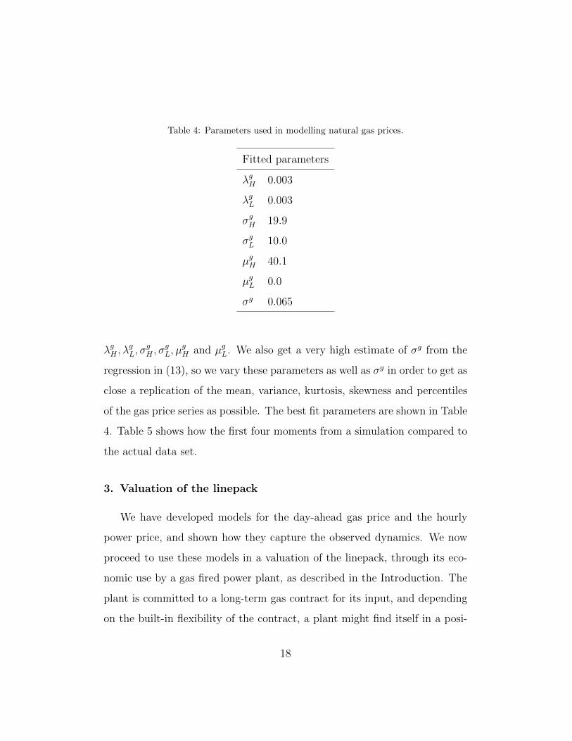
Table 4: Parameters used in modelling natural gas prices.
Fitted parameters
λgH 0.003
λgL 0.003
σgH 19.9
σgL 10.0
µgH 40.1
µgL 0.0
σg 0.065
λgH , λgL, σ
gH , σ
gL, µ
gH and µgL. We also get a very high estimate of σg from the
regression in (13), so we vary these parameters as well as σg in order to get as
close a replication of the mean, variance, kurtosis, skewness and percentiles
of the gas price series as possible. The best fit parameters are shown in Table
4. Table 5 shows how the first four moments from a simulation compared to
the actual data set.
3. Valuation of the linepack
We have developed models for the day-ahead gas price and the hourly
power price, and shown how they capture the observed dynamics. We now
proceed to use these models in a valuation of the linepack, through its eco-
nomic use by a gas fired power plant, as described in the Introduction. The
plant is committed to a long-term gas contract for its input, and depending
on the built-in flexibility of the contract, a plant might find itself in a posi-
18

2
4
8
16
32
64
128
Jun-00 Jun-01 Jun-02 Jun-03 Jun-04 Jun-05 Jun-06 Jun-07 Jun-08 Jun-09 Jun-10 Jun-11
Simulation
NBP
Figure 6: Simulation of gas price compared to the actual gas price. Note that
the simulation only depends on the power price and the previous simulated
price, but it still follows the actual price closely because of the cointegration
with the power price.
19

Table 5: Results of 100 simulations of NBP natural gas prices. The last row, Correlation,
indicates the correlation of the gas price to the 1-week average of the power price.
Period 2000-2011
Actual Simulated
Mean 15.60 16.02
Standard dev. 7.69 7.00
Skewness 2.37 2.14
Kurtosis 12.83 14.72
5% quantile 6.85 7.73
95% quantile 27.4 28.43
Correlation 0.744 0.770
tion where there is little flexibility left. It will have to either produce power
with the committed gas volume or sell it in the spot market. We assume a
scenario where the power plant has little flexibility under the TOP contract.
The situation is the same for a plant that has bought gas on a forward con-
tract. In this scenario, a short-term storage facility such as the linepack may
add value to the power plant. It enables the plant to ramp down production
when the dirty spread becomes negative and ramp up again when it gets
positive—without violating the take obligation. The decision at every point
in time is thus whether to produce power, to sell gas in the market, or to
store it for an a priori unknown time period. The price paid for the gas is
considered a sunk cost, so the gas price used in the decision problem is the
actual spot price at the time of the decision. The stored gas will later be sold
20

for an a priori unknown price, either as gas or converted to electric power.
The choice between the first two options is simple when the efficiency of the
plant is known: If the dirty spread is positive, a unit of gas has higher value
if converted to power, and vice versa. The third option is more complex, as
we discuss below.
In our setup, we assume that the power plant has a fixed, maximum power
output. We assume that the plant can sell all of its power or gas without
influencing prices in the market, disregarding transaction costs and bid-ask
spreads. We discretise time into hours, and assume that the plant can alter
its production instantanously to respond to hourly price changes. In reality
there will be a short period of continuously increasing or decreasing output
while ramping up or down, and there will be costs related to doing this. We
omit these factors to simplify our analysis. If the plant in one specific hour
wishes to sell gas in the market, we will use the settlement price for that day,
modelled in Section 2.2. The settlement price is the weighted average price
for the day, and in absence of rich data on intraday trading we believe this
is a reasonable approximation. Note that this implies a constant gas price
throughout each 24 hour period. We further assume continuous trading of
natural gas contracts also during weekends. We omit any CO2 emission costs,
because this cost will only weakly influence the value of the storage; assuming
that all stored gas will be converted to electricity at some point in time, the
CO2 cost will be paid for all the gas volumes received regardless of the option
of storage.
The linepack has some maximum injection and withdrawal rate, ∆vin and
∆vout, as well as a maximum and minimum storage capacity, vmax and vmin.
21

Taking a real options approach, the value of the option to store gas can be
viewed as a dynamic program. In the Bellman equation (Dixit and Pindyck
[27, p.100]), eq. (14), each state corresponds to a certain point in time, having
a certain volume of gas in the storage, with the prices of gas and power at
a certain level. The control variable is how much to inject or withdraw in
the present state—leading to profits from selling gas or producing power.
For the decision problem of the gas fired power plant, we define the Bellman
equation for the value of the linepack:
Vt(Pt, vt,∆vt) =−∆vtPt + e−ρE[Vt+1(Pt+1, vt+1,∆vt+1)]
Pt ≡max{η · Selt , Sgt }
(14)
where Vt denotes the value of the storage volume at time t, ∆vt the
injection/withdrawal of gas per hour, ρ the discount rate, and η the efficiency
of the plant. The variable Pt, is defined as the maximum of the electricity
price times the plant efficiency and the gas price, i.e., the most profitable
utilisation of the gas. Note that a positive injection to the storage implies
not producing or selling, thereby incurring an alternative cost of ∆vtPt.
3.1. Valuation method: Least Squares Monte Carlo simulation
Following Boogert and de Jong [10], we use LSMC simulation to compute
the value of the linepack. Boogert and de Jong consider a gas storage facility
with large capacity (250,000 MWh) that exploits seasonal and day-to-day
arbitrage opportunities. Our case, on the other hand, has lower storage
capacity, two ways to convert gas withdrawals to money, more complex price
processes, and the opportunity to exploit hourly price patterns. We also
22
perform the storage valuation on the linepack, a volume with more flexible
characteristics than a conventional storage, as discussed in Section 1. We
define a finite period of T hours over which to value the storage. The idea
of LSMC is to simulate M price paths, and at each step along each path
approximate the expected continuation value E[Vt+1(Pt+1, vt+1,∆vt+1)] with
a least squares regression. At time t = 0 and t = T , there must be defined
boundary conditions, for example the volume of gas in the storage at t = 0
and the value of having a certain volume of gas at t = T . To start the
iteration, the values Vt are regressed across all scenarios on the state variables
in the period before. Based on this estimate, the choice is made whether to
inject or withdraw gas, resulting in some realised value Vt−1. The regression
is then repeated for the previous time period.
The regressions used to approximate eq. (14) may have several forms. In
their introduction of the LSMC, Longstaff and Schwartz [11] suggest power
functions, Laguerre polynomials and several other functions of all the state
variables, as well as their cross products. In our application, this would lead
us to regress the values Vt+1 on various terms involving Pt and vt, across
the M price scenarios. However, Boogert and de Jong further discretise the
state space into volume levels, so that Pt is the only independent variable in
the regression. Applying this principle, we are left with a three-dimensional
grid with time t, volume level v and scenario m as the three axes. For a
further discussion of reducing the dimensionality, see Boogert and de Jong
[10]. Based on scatter plots of Vt+1 and Pt for all scenarios, we choose a
polynomial form of order three in the regression.
A Matlab algorithm was written to calculate the value from all allowed
23

injections or withdrawals of gas, and the expected value in eq. (14) is approx-
imated with the regression. It starts at time T and moves backwards, where
the allowed injections and withdrawals are constrained by the maximum and
minimum volume allowed in the storage. Given the boundary condition that
the linepack must be empty at time T and time 0, the value of the linepack is
the average value at time 0 across all simulated price scenarios. When choos-
ing the optimal injection rate ∆vt, it will often be the case that vt + ∆vt is
not a defined point in the grid. In such a case, the expected option value will
be computed as an interpolation between the two closest defined points.
4. Results and discussion
In this section we will use the models developed in Sections 2 and 3 to
create some numerical valuation examples. We will first present a reference
case and analyse the results. The reference case will give an indicative value
on which we can base sensitivity analyses. We proceed to demonstrate how
sensitive the value is to various parameters, and how the optimal dispatching
change when the parameters vary. Consider a medium sized combined cycle
plant with a maximum power output of 300MW and efficiency of 53.8%4. We
assume it receives 200MWh of gas per hour, corresponding to the parameter
vin, and that it is allowed to store gas in the linepack for up to 10 hours, i.e.,
vmax is 2000MWh. The maximum gas withdrawal vout is −100MWh, such
that all the incoming gas and the withdrawals total to the maximum output
of 300MW. We simulate 1000 price scenarios of three weeks length, and use
4The efficiency corresponds to a General Electric LMS100 combined cycle gas turbine.
24

Table 6: Parameters used in reference case.
vmax 2000 MWh
vmin 0 MWh
η 53.8 %
vin 200 MWh
vout -100 MWh
T 504 hours ( = 3 weeks)
ρ 6%
M 1000 simulations
an annual, exogenous discount rate of 6%. These parameters are summarised
in Table (6).
Recall the assumption that the power plant is in a situation with little
or no flexibility left in the take-or-pay contract, meaning that without any
storage option it has to use or sell all the incoming gas. The prices are
simulated over three weeks, as it is unlikely that a power plant will be in this
situation for very long periods of time. We use a discretisation of N = 100
volume levels, meaning that each volume step will be 20 MWh for vmax =
2000. We first show how the production and storage decisions vary with the
prices of the input variables. Consider Figure 7. We see that whenever the
price is low, production ceases and gas is stored. When either the gas price
is higher than normal or the storage volume is full, gas is sold on the market.
Notice that at around t = 175 hours, the power price spikes downwards while
the storage volume is full. The power plant will sell no more than the gas
25

received each hour, as the probability of higher power prices in the future
makes it suboptimal to empty the storage.
0 25 50 75 100 125 150 175 200 225 250 275 300 325 350 375 400 425 450 475 500
−300
−200
−100
0
100
200
300
0 25 50 75 100 125 150 175 200 225 250 275 300 325 350 375 400 425 450 475 5000
10
20
30
40
50
0 25 50 75 100 125 150 175 200 225 250 275 300 325 350 375 400 425 450 475 5000
500
1000
1500
2000
Production (black bar) and gas sales (grey bar)MW
Prices: Power price (dotted line), gas price (grey line), realised price (black line)EUR/MWh.
Storage utilisationMWh.
.
Figure 7: Simulation of three weeks of storage and production. Top: Produc-
tion and gas sales in MW. Positive values imply production, negative (grey)
values imply that gas is sold in the market. Middle: Price series of power and
gas. The grey series is the daily gas price, the dashed line is the hourly power
price corrected for efficiency, and the continuous line is the P (t), meaning
the maximum of these two. Bottom: Storage volume in MWh. Horizontal
axis in hours.
26

The value of a license to use the linepack over a period of three weeks is
estimated to 249,234 euro. This reference case scenario value is computed
taking the average of ten runs of M = 1000 simulations each run. The
standard deviation of the ten computed values is 427 euro. If we assume
no access to linepack storage, the plant would have to produce power or sell
gas at market prices every hour. Computing the revenue of the same period
without a storage option reveals that the linepack value is about 8.5% of this
revenue. Even more interesting is the increase in profitability. The cost of gas
in take-or-pay contracts is usually confidential, but if we assume a constant
gas price of 22 EUR/MWh and that the plant has no other costs, its profit
would increase by 34% during the period of time in which the plant has a
low flexibility due to commitment to a TOP or forward contract. Converted
to power price terms, this corresponds to an increase of 2.51 EUR/MWh
over the simulated period. The reference case assumes no trading, ramp-
up or ramp-down costs for the power plant. As the algorithm calculates
the isolated value of being able to store gas, we conclude that the increased
flexibility indeed can be considered valuable to a plant in a situation of low
initial flexibility. The storage option allows for better utilisation of gas and
increased profits to the owners of the plant. The results shown imply that
a broader utilisation of the linepack in the pipeline network would enable
more efficient operation of power plants; potentially even dampening the
extreme spikes seen in today’s power prices. By a no-arbitrage argument,
if every plant had the same flexibility, some of the variation in prices could
be eliminated. The price volatility is the primary source of profits for the
storage volume as a separate entity, so an increased use of the linepack would
27

also reduce the marginal value of each MWh of storage volume. However, it
may be a valuable tool for the energy system as a whole.
Below we show some examples of how sensitive the value of the linepack
is to changes in parameters of the storage volume or the price processes. In
each simulation we use M = 250 simulations.
-
50,000
100,000
150,000
200,000
250,000
300,000
350,000
1 2 4 8 16 32 64 128 256 512 1024 2048
vmax - Maximum storage volume (GWh)
N = 1000
N = 600
N = 400
N = 200
N = 100
Figure 8: A higher storage volume (vmax) requires a higher volume discreti-
sation (N) to provide a good estimate. For N = 100, the value of a 64 GWh
storage volume is estimated to be lower than for a 32 GWh volume. For
N = 1000, the value is equal, as one would expect.
We now analyse how the value changes with increased storage capacity.
When evaluating how the value of the linepack varies with the maximum stor-
age capacity vmax, one would expect that the value at first increases rapidly
with higher capacity, but that it eventually flattens out as the capacity goes
to infinity. One could say that when value goes to infinity, flexibility only
goes to 100%, and asymptotically the value should also reach a maximum.
We find that for low values of volume levels N with high values of vmax,
the asymptotic value of the storage volume actually falls (Figure 8). This is
caused by the error of interpolation increasing with higher capacity as the
28

LSMC algorithm divides the maximum volume into N+1 levels. An interpo-
lation is a linear function while our model estimates the value of continuation
by a polynomial function of power 3, rendering the interpolation inaccurate
for large intervals. We observe that for higher volume discretisation (higher
N), the accuracy improves and the value goes asymptotically to a stable
level as the volume rises. We can see from Figure 8 that for N = 100 and
vmax = 4000 the error of estimation is small, while for vmax = 8000 it is vis-
ible. We can conclude that the size of N relative to vmax should be around
140
.
In Section 2, we estimated the parameters of our price models and noted
some potential estimation errors, most notably in the gas price model. We
now address the sensitivity of the value estimate to changes in different pa-
rameters. None of the parameters in the gas price model showed significant
effect on the value, as it is seldom optimal to sell gas in the market. The
results from gas price sensitivity analyses is therefore omitted. However,
Europe may expect a larger fraction of renewable power generation in the
future. Germany is phasing out its nuclear power plants and the UK has
ambitious goals for wind power. Both solar and wind power has relatively
unpredictable and volatile output, and we therefore analyse how changes in
power price volatility and spike occurences affect the linepack value. This
corresponds to the parameters σel, λelH and λelL , as well as pML and pMH (the
last two representing the frequency of the power price entering the spike
regimes).
Figures 9 and 10 show the effect of the variation in parameters on the
estimate of the value. Higher values of both σel and the arrival rates of spikes
29

increase the overall volatility of the power price, implying that power price
volatility is the main value driver for the linepack. Analysing Figure 11,
the effect from changes in pML, one can see that more spikes to the low
regime increases the value of the linepack more than λH and λL. The implicit
price increase from increases in pMH is not that relevant, because high spikes
increase revenue along with the linepack value.
2.00
2.20
2.40
2.60
2.80
3.00
3.20
3.40
0.02 0.04 0.06 0.08 0.10 0.12 0.14 0.16 0.18 0.20 0.22 0.24 0.26 0.28 0.30 0.32 0.34 0.36 0.38 0.40
EUR/MWh
σel
Reference case
Figure 9: Implicit power price increase when varying volatility σel in the
power price. In the reference case, σel = 0.21.
5. Conclusion
Linepack is an under-utilised and under-communicated short-term energy
storage option. Since it uses existing natural gas pipeline infrastructure, it is
cost efficient and environmentally sound. In this article we have analysed its
value for a participant in the natural gas value chain. We exemplified the idea
through a gas fired power plant, facing both gas price and electricity price
volatility. We developed models for power and gas prices that can accurately
30

2.30
2.35
2.40
2.45
2.50
2.55
2.60
2.65
2.70
0.0 0.5 1.0 1.5 2.0 2.5 3.0 3.5 4.0
EUR/MWh
λL
2.30
2.35
2.40
2.45
2.50
2.55
2.60
2.65
2.70
- 0.5 1.0 1.5 2.0 2.5 3.0 3.5 4.0
EUR/MWh
λH
Reference case Reference case
Figure 10: Implicit power price increase when varying arrival rates λelH and λelL
for high and low spikes in the power price. In the reference case, λelH = 1.89
and λelL = 1.84.
2.3
2.35
2.4
2.45
2.5
2.55
2.6
2.65
2.7
0.0001 0.02 0.04 0.06 0.08 0.1 0.12 0.14 0.16 0.18
EUR/MWh
pML
Reference case
Figure 11: Implicit power price increase when varying pML in the power
price. In the reference case, pML = 0.044.
capture both regular variations, irregular spikes, and the covariation in the
two prices. The Least Squares Monte Carlo algorithm was employed in the
valuation, and we conclude that the flexibility of having a storage opportunity
31

was indeed beneficial for the power plant. Specifically, when committed to a
take-or-pay contract, the plant in the reference case could increase the value
of the gas by 34% with the option to store gas for up to ten hours. This
is equivalent to receiving a power price that is 2.51 EUR/MWh higher than
market prices, over the three week period simulated. Further, we showed that
the volatility and spike arrival rates of the power price are the most significant
value drivers, because in most cases storing gas to produce power later is
more profitable than selling gas in the market. The gas price parameters are
therefore of smaller importance. The capacity of linepack storage increases
value up to a limit where no more flexibility is used. In a future with more
output from unpredictable renewable power sources, such as solar and wind
power, the linepack may enable participants in the natural gas value chain
to more efficiently utilise its gas.
References
[1] The Interstate Natural Gas Association of America (INGAA), Natural
gas pipeline and storage infrastructure projections through 2030, 2009.
INGAA and ICF International Report, Washington DC, USA.
[2] X. Sun, D. Huang, G. Wu, The current state of offshore wind energy
technology development, Energy 41 (2012) 298–312.
[3] S. Lochner, Identification of congestion and valuation of transport in-
frastructures in the European natural gas market, Energy 36 (2011)
2483–2492.
[4] P. Osmundsen, T. Aven, A. Tomasgard, On incentives for assurance of
32

petroleum supply, Reliability Engineering & System Safety 95 (2010)
143–148.
[5] International Energy Agency (IEA), Natural gas information, 2010.
OECD and International Energy Agency Report, Paris, France.
[6] H. Tan, Y. Li, H. Tuo, M. Zhou, B. Tian, Experimental study on
liquid/solid phase change for cold energy storage of liquefied natural gas
(LNG) refrigerated vehicle, Energy 35 (2010) 1927–1935.
[7] K. Midthun, M. Nowak, A. Tomasgard, An operational portfolio op-
timization model for a natural gas producer, in Optimization models
for liberalized natural gas markets (K. T. Midthun), PhD thesis NTNU,
Trondheim, Norway (2007).
[8] M. Chaudry, N. Jenkins, G. Strbac, Multi-time period combined gas
and electricity network optimisation, Electric Power Systems Research
78 (2008) 1265–1279.
[9] N. Keyaerts, M. Hallack, J. Glachant, W. Dhaeseleer, Gas market dis-
torting effects of imbalanced gas balancing rules: Inefficient regulation
of pipeline flexibility, Energy Policy 39 (2011) 865–876.
[10] A. Boogert, C. de Jong, Gas storage valuation using a Monte Carlo
method, Journal of Derivatives 15 (2008) 81–91.
[11] F. Longstaff, E. Schwartz, Valuing American options by simulation: A
simple least-squares approach, Review of Financial Studies 14 (2001)
113–147.
33

[12] G. Lai, M. Wang, S. Kekre, A. Scheller-Wolf, N. Secomandi, Valuation
of storage at a liquefied natural gas terminal, Operations Research 59
(2011) 602–616.
[13] P. Bjerksund, G. Stensland, F. Vagstad, Gas storage valuation: Price
modelling v. optimization methods, The Energy Journal 32 (2011) 203–
228.
[14] J. Husebye, R. Anantharaman, S.-E. Fleten, Techno-economic assess-
ment of flexible solvent regeneration storage for base load coal-fired
power generation with post combustion CO2 capture, Energy Proce-
dia 4 (2011) 2612–2619.
[15] C. A. Kang, A. R. Brandt, L. J. Durlofsky, Optimal operation of an
integrated energy system including fossil fuel power generation, CO2
capture and wind, Energy 36 (2011) 6806–6820.
[16] S. van Dyken, B. H. Bakken, H. I. Skjelbred, Linear mixed-integer
models for biomass supply chains with transport, storage and processing,
Energy 35 (2010) 1338 – 1350.
[17] C. de Jong, The nature of power spikes: A regime-switch approach,
Studies in Nonlinear Dynamics & Econometrics 10 (2006) 61–88.
[18] J. Janczura, R. Weron, Efficient estimation of Markov regime-switching
models: An application to electricity spot prices, Advances in Statistical
Analysis 96 (2012) 385–407.
[19] S. Schneider, Power spot price models with negative prices, 2010. MPRA
paper No. 29958.
34

[20] L. Abadie, J. Chamorro, Monte Carlo valuation of natural gas invest-
ments, Review of Financial Economics 18 (2009) 10–22.
[21] N. Secomandi, On the pricing of natural gas pipeline capacity, Manu-
facturing & Service Operations Management 12 (2010) 393–408.
[22] A. Siddiqui, C. Marnay, Distributed generation investment by a micro-
grid under uncertainty, Energy 33 (2008) 1729–1737.
[23] S.-E. Fleten, K. Maribu, I. Wangensteen, Optimal investment strategies
in decentralized renewable power generation under uncertainty, Energy
32 (2007) 803–815.
[24] C. Won, Valuation of investments in natural resources using contingent-
claim framework with application to bituminous coal developments in
Korea, Energy 34 (2009) 1215–1224.
[25] J. Hamilton, Analysis of time series subject to changes in regime, Jour-
nal of Econometrics 45 (1990) 39–70.
[26] C. de Jong, S. Schneider, Cointegration between gas and power spot
prices, The Journal of Energy Markets 2 (2009) 27–46.
[27] A. K. Dixit, R. S. Pindyck, Investment Under Uncertainty, Princeton
University Press, Princeton, NJ, 1994.
35