MPRAMunich Personal RePEc Archive

Family size, human capital and growth:structural path analysis of Rwanda

Tugrul Temel

Development Research Institute (IVO), Tilburg University

21 June 2011

Online at https://mpra.ub.uni-muenchen.de/31741/MPRA Paper No. 31741, posted 21 June 2011 14:15 UTC

IVO Working Paper 11-06Family size, human capital and growth:structural path analysis of Rwanda

Tugrul TemelDevelopment Research Institute

Tilburg University, The Netherlandst.temel@uvt.nl

June 15, 2011

Abstract

This paper analyzes the role that different household groups playin human capital formation, sectoral growth and income distribution inRwanda. Using the 2006 SAM of Rwanda, the paper calculates accountingmultipliers to characterize the transmission of economic influences stim-ulated by an exogenous income injection. The paper further exploresmacroeconomic implications of family size for human capital, sectoralgrowth and income distribution, drawing on the pathways identified bystructual path analysis. The following two findings are noted. First, thesmaller the number of children in an average family, the higher the in-vestment in human capital of the children in that family, demonstratingthe presence of quantity-quality trade-off. In particular, the householdgroup with 1-3 children tends to spend more for the improvement of ed-ucation and health status of children than those household groups withmore than 3 children. Second, an improvement in human capital leadsto a significant increase in agricultural production and that householdswith 1-3 children act as an important intermediate pole transmitting theinfluence of human capital investment on agricultural production. In con-clusion, promoting family planning programs in Rwanda thus seems to bea viable strategy for economic growth and poverty reduction, consideringthe current average family size of 5 children.

1

1 Background and Introduction

The role of human capital in economic growth and development has been welldocumented in the literature.1 The debates about the relationship betweenhuman capital and economic development evolve around three main assertions(Rosenzweig, 1988; Bloom, Canning and Sevilla, 2001). First, large familiesdirectly contribute to lowering human capital; for given resources, high fertil-ity impedes human capital formation. Dissemination of information to familiesabout the negative consequences of high fertility for their children and provid-ing the means for controlling fertility should be high priorities for public agen-cies. Second, human capital investment reflects the economic circumstances of acountry; the observed mix of large families and low levels of education, health,and nutrition are symptoms, not causes, of a lack of economic development.Governments and international development agencies should therefore focus onremoving impediments to economic development and not on families’decisionsabout their family size. Third, the inability to control fertility is an importantdeterrent to human capital investment. These assertions clearly demonstratethat fertility and poverty are interlinked through investment in human capitalnot only at the household but also at the national level. Considerable evidencefrom the development literature suggests that lowering fertility - in part throughfamily planning programs - is essential to reduce population growth, increase percapita income through investment in human capital and hence reduce povertythrough good policies.The Rwandan government has formally acknowledged the link between fer-

tility and poverty (MINECOFIN, 2007) and embarked on various large-scale,donor-funded family planning programs (Solo, 2008).2 The contribution of theseprograms and supportive policies to the smooth transition to stability and de-velopment cannot be overlooked. Demographic programs during the period of1995-2006 have led to an average fertility rate of about five, while economicpolicy has led to an average GDP growth of 7.3 percent per year. The sectoralcontribution to this high economic growth during the period concerned hasbeen researched by a large number of studies in the literature (see Diao, Fan,Kanyarukiga and Yu, 2010); however, the extent to which different householdgroups transmit the economic influence of an exogenous income injection ontothe economy-wide human capital formation, employment, output and incomedistribution remains largely unexplored. This paper aims to shed light on the

1Human capital theory focuses on education and health as inputs to economic growth anddevelopment. Human capital is a broad concept, which includes peoples’ knowledge, skills,strength and vitality, acquired partly by education and partly by health and nutrition. Schütt(2003) presents a comprehensive review of selected theoretical models of human capital andeconomic growth, discussing the empirical findings and their policy implications from a largenumber of studies.

2Rwanda has a young population, with a mean age of 21 years, and children under 15comprise 43% of the population. The average household has 5 members. Nationally, everyworking person supports 1.2 persons; for the poorest households this is 1.5 and for the richestit is 1. Increasing GDP offers a window of opportunity for investing in education, health andnutrition of the children and paves the way for healthy and more skilled labor to increaseproductivity.

2

role of family size in the transmission of economic influences during the period1995-2006. In order to facilitate the analysis of the linkages between familysize and human capital formation, the 2006 Social Accounting Matrix (SAM)of Rwanda has been adjusted. The first adjustment is the disaggregation ofhousehold account into 4 groups: household group 1 includes those householdswithout children; group 2, with 1-3 children; group 3, with 4-5 children; andgroup 4, with more than 5 children. The second adjustment is the disaggre-gation of both production and commodity accounts into 5 sectors: agriculture,manufacturing, service, education and health sectors. In the context of the cur-rent paper, the education and health sectors together are assumed to reflect thedevelopments concerning human capital formation.In the literature, analysis of the economic effects of fertility usually focuses on

an assessment of the rate of return to investment in human capital because highfertility puts mothers at risk, rises the dependency ratio and lowers per childinvestment in human capital, which in turn at the macro level reduces productiv-ity and income. A large number of micro-econometric and demographic studiesshow that family size is negatively correlated with children’s educational andhealth attainment (see, for example, Rosenzweig and Wolpin, 1986; Rosenzweig,1988; Angrist, Lavy and Schlosser, 2005; Schultz, 2005; Rosenzweig and Zhang,2009). Many studies also suggest that providing family planning services isthe most direct and effective way to reduce fertility, making other interventionsmore effective in improving overall welfare (for example, World Bank, 1990;Ross, Parker, Green and Cooke, 1992; Schultz, 1997). Complementing microstudies are macroeconomic analyses which integrate household fertility behav-ior with the consumption/saving decision. The models presented by Beckerand Barro (1988) and Barro and Becker (1989), for example, demonstrate thatfertility is inversely related to growth. At low levels of education, a combina-tion of low productivity and high fertility point to a Malthusian equilibrium.With a general equilibrium model, Becker, Murphy and Tamura (1990) derivesthe conditions under which a country may switch from the Malthusian to the"development" equilibrium in which high levels of human capital stock lead tohigh productivity and low fertility. Their analysis highlights that a countrymay reach a reasonably high development level if it has good policies that favorhuman capital investment. More recently, the focus switched towards modelsthat discuss demographic transition and offer diverse explanations (e.g., Galorand Weil 1996, 2000). Azarnert (2004) introduced an analysis of interactionsbetween income redistribution, fertility and growth in an open economy. Thelist can be extended at will.The literature has not been so generous in the analysis of economy-wide ef-

fects of households or family size within SAM framework, although such analy-sis may provide critical information on effective targeting of specific householdgroups. So far, only a few studies have been carried out.3 For example, Defourny

3On the contrary, there is a large number of studies applying the SAM multiplier methodto analyze: growth strategies in developing economies (Pyatt and Round, 1985), incomedistribution and redistribution (Pyatt and Thorbecke, 1976; Roland-Holst and Sancho, 1992),fiscal policies (Whalley and Hillaire, 1987), intersectoral linkages and poverty (Thorbecke,

3

and Thorbecke (1984) characterize the interactions among production, factorsof production and households in the context of South Korea. They demon-strate that when production activities are poorly linked, households facilitatethe transmission of economic influence across production activities. Likewise,Roberts (1996) finds out that households play an important role in the estab-lishment and strengthening of structural linkages between agriculture and therest of the economy as well as in the rural-urban spillover. Examining the role ofdifferent household groups in the transmission of exogenous shocks within ruraleconomies, Roberts (2005) further demonstrates that households with childrenare the most important transmitters of economic influence within the local econ-omy examined and that large differences exist with respect to the dependenceof different sectors on particular types of households. Another original studyfollows from Osorio, Carlos and Quentine (2010), adopting the SAM framework,explores the transmission channels through which sectoral growth patterns ofTanzania imply different effects on the incomes of women and men. The findingsobtained are illustrative in nature rather than informing policies. The currentpaper intends to provide a case study of Rwanda, applying the structural pathanalysis (SPA) to identify critical pathways from households to human capitalformation (i.e., education and health) and from human capital production toother production sectors.4 This would not only uncover the actual sources ofthe multiplier effects but also demonstrate the welfare-improving sequence ofpolicy interventions.The following findings seem to emerge from our analysis. First, there is a

trade-off between family size and human capital formation: the higher the num-ber of children, the less the investment in human capital of the children. Morespecifically, the evidence reveals that household groups with up-to three childrentend to spend more for the improvement of the education and health status oftheir children than those household groups with more than three children. Sec-ondly, the path analysis reveals that an improvement in human capital promisesa significant growth of agricultural production and that households with upto3 children act as an important intermediate pole transmitting the influence ofhuman capital investment on agricultural growth in particular and on the restof the economy in general. These two findings together suggest that promotingfamily planning programs and policies in Rwanda seems to be a viable strat-egy for economic growth and poverty reduction, considering the current averagefamily size of 5 children.The scenario analysis provides additional evidence that investing in educa-

tion and health is the first best policy in terms of net aggregate income gain.Regarding the sectoral income and employment effects, a relatively higher in-vestment in education paves the way for: (i) the H0, the H13 and Pa to absorba significant portion of the income gains made and (ii) a higher level of laborand capital employment relative to the employment from an equivalent invest-

1995) among many others.4The reader is referred to the following methodology papers: Defourny and Thorbecke

(1984), Khan and Thorbecke (1989), Round (2003), Thorbecke (1995) and Thorbecke andJung (1996).

4

ment in the health sector. Furthermore, a comparison of Scenario [1] with [17]demonstrates a striking result that investing in education and health is welfareimproving over investing in the agricultural and manufacturing sectors and thatinvesting in education and health leads to higher household income. Finally, thebackward-forward linkage analysis reveals that the health and education sectorsare the key sectors of the economy, promoting growth in the rest of the economy.The rest of the paper is organized as follows. Section 2 presents the SAM

multiplier and structural path analysis of Defourny and Thorbecke (1984). Sec-tion 3 describes how the original SAM has been adjusted to facilitate the analysisof the linkages between four household groups and the rest of the economy. Thekey empirical findings and their policy implications are discussed in Section 4.Section 5 concludes the paper, with a summary of the main results.

2 Methodology

2.1 Multiplier analysis

SAM is a matrix representation of the system of national accounts. In a SAM,column sums (i.e., expenditures) are equal to row sums (i.e., incomes). Toanalyze a policy change, some accounts in the SAM must be manipulable ex-ogenously; therefore, in a modeling framework, the SAM is partitioned as en-dogenous and exogenous accounts. Production activities, commodities, factors,households and firms represent endogenous accounts, while the government,savings-investment and the rest of the world accounts are assumed to be exoge-nous.Let T(d,d) = [tij ]i=j=1,...,d denote a SAM with d = (n + x) where n and

x denote the number of endogenous and exogenous accounts, respectively. Anelement, tij , represents account j’s expenditure on the output from account i.Let T(d,d) be partitioned as:

T(d,d) =

[Tnn TnxTxn Txx

]

where Tnn = transactions among endogenous accounts

Tnx = injections from exogenous into endogenous accounts

Txn = leakeges from endogenous into exogenous accounts

Txx = residuals arising from interactions among exogenous accounts

(N,X,L,R) = vectors of row sums of (Tnn, Tnx, Txn, Txx), respectively

y = (y1, ..., yd) ≡ ((yn), (yx)) = vector of row sums of T(d,d)y′ = (y′1, ..., y

′d) ≡ ((y′n), (y′x)) = vector of column sums of T(d,d)

Let A(d,d) = [aij ]i=j=1,...d denote a matrix of average expenditure propensi-

ties (AEPs) where aij = (tij/y′j) and

d∑i=1

aij =d∑i=1

(tij/y′j) = 1 for ∀j=1,2,...,d .

5

Let A(d,d) be partitioned as:

A(d,d) =

[Ann AnxAxn Axx

](2)

where Ann is a square matrix of AEPs across n endogenous accounts; Axn is amatrix of leakages; that is, the proportions of n endogenous accounts that leakout as expenditure into x exogenous accounts; Anx is a matrix of injections;that is, the proportions of expenditures of x exogenous accounts injected into nendogenous accounts; and Axx is a matrix of residuals; that is, the proportionsof expenditures circulated only among x exogenous accounts.

SAM accounting multiplier matrix, Mnn, follows from:

yn = N +X = Annyn +X

= (I −Ann)−1X= MnnX. (3)

For notational convenience, from now on, we drop the subscript n from Mnn.The multiplier matrix M = (dyn/dX) = (I − Ann)−1 measures the impact ofunit change in aggregate demand, X, on the incomes of endogenous accounts,yn.5

There are two ways to conduct scenario analysis. The simplest and mostcommonly applied way is to deal with only one target ("sink": point of finaleffect) and one instrument ("source": point of injection). Eq. (3) represents themodel used for the analysis of a single, aggregate injection. A more complexmodel given in Eq. (4) is used to deal with multiple targets and multiple instru-ments. Replacing X in Eq. (3) with Tnx allows us to disentagle the individualimpacts of multiple injections originating from several exogenous accounts:

ynx =MTnx (4)

where ynx is a matrix of n rows and x columns. Each column in ynx representsthe vector of endogenous incomes associated with a single exogenous accountsuch as the government.

2.2 Structural path analysis

The SPA is based on two types of paths. The first type is a direct-binarypath given in Eq. (5), linking two accounts without any intermediate account.A′(n,n) is a matrix of direct-binary paths and the expenditure propensities in itcorrespond to economic influences.6 Take, for example, the direct-binary path,

5See Defourny and Thorbecke (1984) for the implication of unitary income elasticity andfor the linkages between accounting and fixed-price multipliers. The lack of data on expen-diture (income) elasticities does not allow us to compute marginal expenditure propensitiesassociated with the SAM of Rwanda.

6 It should be noted that the path analysis is carried out using A′(n,n)

, which is the transpose

of A(n,n). With this convention, the elements in a row in A′(n,n)

represent the expenses ofthe corresponding account, while the elements in the corresponding column represents theincome. Therefore, aij in A′(n,n) would define the influence from account i to j.

6

ID(i→ j), indicating the actual influence, aij ∈ A′(n,n), transmitted from row ito column j:

ID(i→ j) = aij︸︷︷︸influence of i on j

(5)

The second type is a direct pathway p given in Eq. (6), linking two accounts(i and j) through one or more intermediate accounts. The direct influence,ID(i → j)p, transmitted through this pathway p with intermediate accountsk, z,and u is defined:

ID(i→ j)p = ID(i, k, z, u, j) = aikakzazuauj︸ ︷︷ ︸

influence of i on j through k, z and u

(6)

For illustrative purposes, let (i, k, z, u, j) represent the direct pathway p = 1between i and j. The level of influence actually transmitted through p = 1 isestimated as the multiplication of direct, binary path expenditure propensities:(aikakzazuauj).

It should be noted that the direct influences explained above do not coverthe influences implied by possible adjacent feedback circuits. The measure oftotal influence from i to j in Eq. (7) does the job, encompassing all of thepossible indirect effects implied by these feedback curcuits. Suppose that thereare two feedback curcuits associated with the direct pathway (i, k, z, u, j): onefrom u back to k denoted by (u → k) and another from k back to i through anew account r denoted by (k → r → i). In this case, the total influence of p = 1is computed as:

IT (i → j)1 = IT (i, k, z, u, j) (7)

= ID(i, k, z, u, j)M1 = (aikakzazuauj)M1

where the path multiplier M1 estimates the degree to which the direct influencealong the direct pathway (i, k, z, u, j) is amplified through the effects of the twofeedback curcuits {(u→ k), (k → r → i)}. M1 is calculated as (41/4) where4is the determinant | I −Ann | of the structure represented by Tnn and 41is thedeterminant of the structure excluding the accounts (i, k, z, u, j) constitutingthe pathway p = 1.It is very likely to have more than one pathway spanning from i to j̇. Suppose

that two other pathways exist between i and j : (i, s, j) and (i, v, j) with a looparound v. The total influences of these additional pathways are, respectively,calculated as:

IT (i → j)2 = IT (i, s, j) = ID(i, s, j)M2 = (aisasj)M2

IT (i → j)3 = IT (i, v, j) = ID(i, v, j)M3 = (aivavj)M3

7

Finally, global influence from i to j is defined as:

IG(i → j) = mij =

3∑p=1

ITp (i→ j) =

3∑p=1

IDp (i→ j)Mp (8)

= IT (i→ j)1 + IT (i→ j)2 + I

T (i→ j)3

= ID(i→ j)1M1 + ID(i→ j)2M2 + I

D(i→ j)3M3

= ID(i, k, z, u, j)M1 + ID(i, s, j)M2 + I

D(i, v, j)M3

= (aikakzazuauj)M1 + (aisasj)M2 + (aivavj)M3

For notational convenience, in the SPA we use mij ∈ M ′ where M ′ is thetranspose of M.

2.3 Data

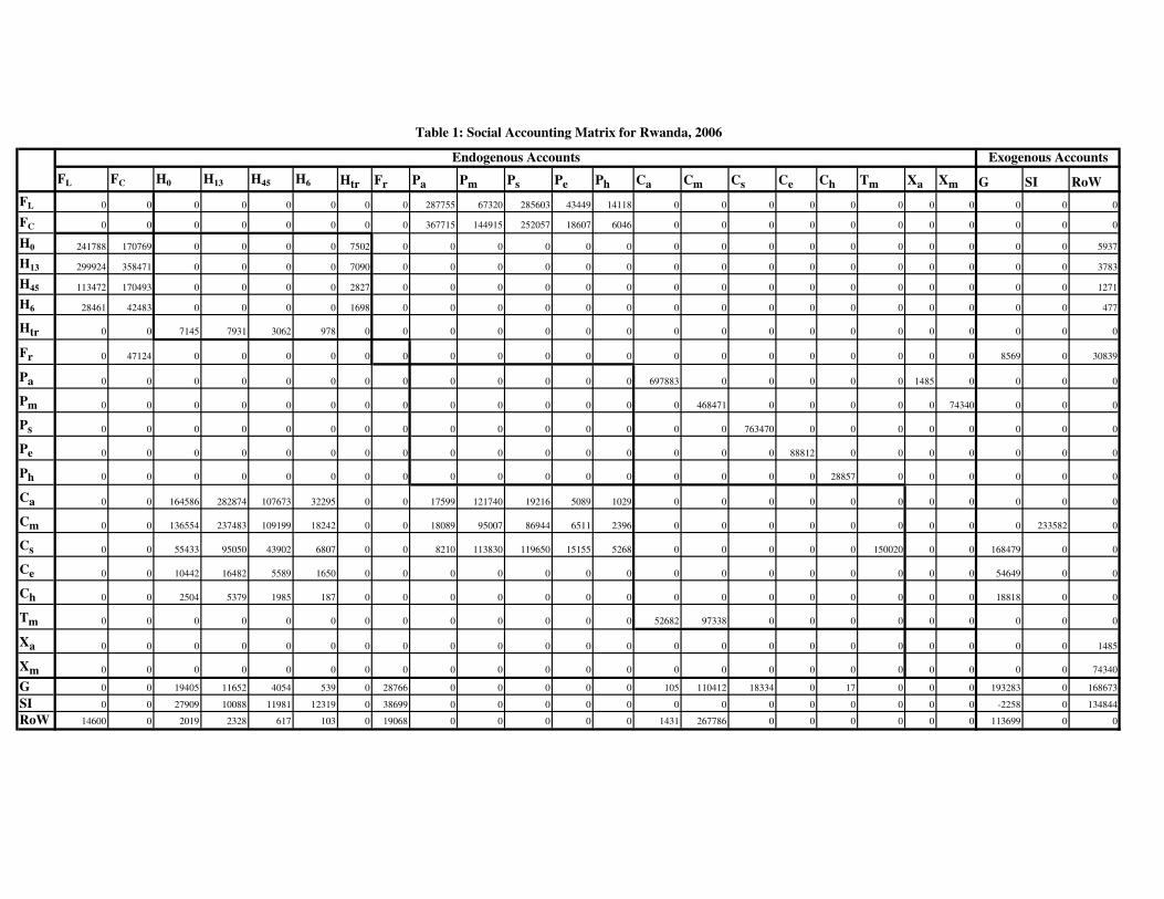
Emini (2007) has compiled the only available SAM for Rwanda, using the 2006data. This SAM with 197 accounts has been revised by reducing its dimensionto 24 accounts: 2 factors of production, 4 household groups plus 1 householdtransfer account, the firms account, 5 production activities, 5 commodities plus1 trade margin account, 2 exportable commodities, the savings account, the gov-ernment account and the rest of the world account (Table 1). For the purposeof our analysis, the household account has been adjusted to create 4 householdgroups based on the number of children (15 years old or younger). Householdgroup 1 includes those households with no children; group 2, with 1-3 children;group 3, with 4-5 children; and group 4, with more than 5 children. Consideringthe observation that the current average fertility rate in Rwanda is about 5 chil-dren, the grouping concerned allows us to compare the human capital formationbehaviour of households in Groups 1 and 2 with those in Groups 4 and 5. Sucha grouping also allows us to characterize the behavior of a specific householdgroup with respect to its human capital formation in particular and the roleof households in the transmission of economic influence in the Rwandan econ-omy in general. The production account has been aggregated into 5 activities,including agriculture, manufacturing, services, education and health.The revision of Emini’s original SAM has required a substantial amount

of data compilation using the 2005-2006 household living conditions survey(EICV2) (MINECOFIN, 2007). In the construction of 4 household groups, usingall the variables listed in Table 8 of Emini (2007), we have organized the EICV2data to construct household-group specific incomes and expenditures across the24 accounts of the SAM. Expectedly, the row and column sums in the revisedSAM were not consistent (i.e., row sums were not equal to column sums) dueto the fact that the EICV2 survey data were obtained from a sample of 6900households only. In order to construct a consistent SAM, the household-groupspecific percentages calculated from the EICV2 data were repeatedly applied tothe aggregate figures given in Emini’s original SAM.An important issue to note is that the survey does not provide child-specific

health and education data but rather provides the desired data at the household

8

level. This means that, given a household group, the health and educationexpenses in the SAM should be read as that household group’s gross health andeducation expenses, not necessaily as the expenses on the children falling underthat household group.

3 Key findings

This section presents the key findings from the multiplier and path analyses,with a special focus on the role that different household groups play in thehuman capital formation, sectoral growth and income distribution in Rwanda.

3.1 Multiplier analysis

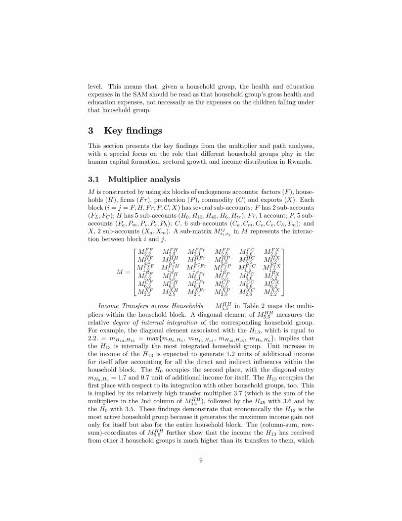
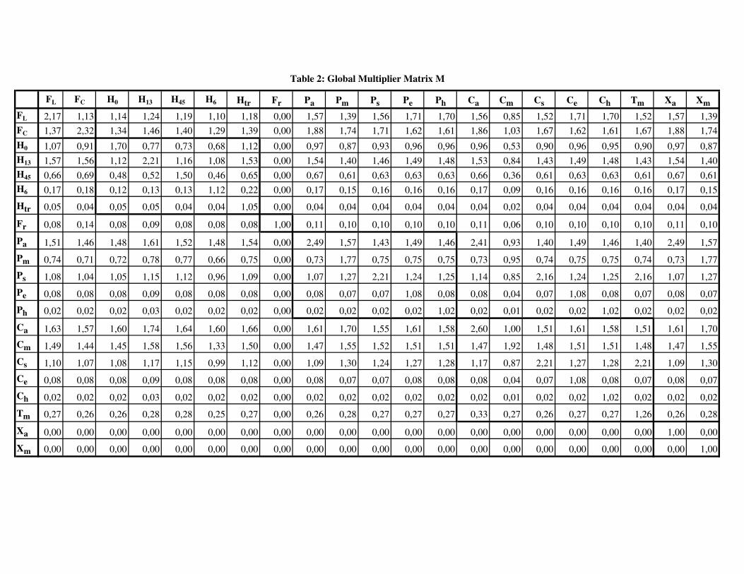
M is constructed by using six blocks of endogenous accounts: factors (F ), house-holds (H), firms (Fr), production (P ), commodity (C) and exports (X). Eachblock (i = j = F,H, Fr, P, C,X) has several sub-accounts: F has 2 sub-accounts(FL, FC); H has 5 sub-accounts (H0, H13, H45, H6, Htr); Fr, 1 account; P, 5 sub-accounts (Pa, Pm, Ps, Pe, Ph); C, 6 sub-accounts (Ca, Cm, Cs, Ce, Ch, Tm); andX, 2 sub-accounts (Xa, Xm). A sub-matrix M ij

si,sj in M represents the interac-tion between block i and j.

M =

MFF2,2 MFH

2,5 MFFr2,1 MFP

2,5 MFC2,6 MFX

2,2

MHF5,2 MHH

5,5 MHFr5,1 MHP

5,5 MHC5,6 MHX

5,2

MFrF1,2 MFrH

1,5 MFrFr1,1 MFrP

1,5 MFrC1,6 MFrX

1,2

MPF5,2 MPH

5,5 MPFr5,1 MPP

5,5 MPC5,6 MPX

5,2

MCF6,2 MCH

6,5 MCFr6,1 MCP

6,5 MCC6,6 MCX

6,2

MXF2,2 MXH

2,5 MXFr2,1 MXP

2,5 MXC2,6 MXX

2,2

Income Transfers across Households – MHH

5,5 in Table 2 maps the multi-pliers within the household block. A diagonal element of MHH

5,5 measures therelative degree of internal integration of the corresponding household group.For example, the diagonal element associated with the H13, which is equal to2.2. = mH13,H13

= max{mH0,H0, mH13,H13

, mH45,H45, mH6,H6

}, implies thatthe H13 is internally the most integrated household group. Unit increase inthe income of the H13 is expected to generate 1.2 units of additional incomefor itself after accounting for all the direct and indirect influences within thehousehold block. The H0 occupies the second place, with the diagonal entrymH0,H0

= 1.7 and 0.7 unit of additional income for itself. The H13 occupies thefirst place with respect to its integration with other household groups, too. Thisis implied by its relatively high transfer multiplier 3.7 (which is the sum of themultipliers in the 2nd column of MHH

5,5 ), followed by the H45 with 3.6 and bythe H0 with 3.5. These findings demonstrate that economically the H13 is themost active household group because it generates the maximum income gain notonly for itself but also for the entire household block. The (column-sum, row-sum)-coordinates of MHH

5,5 further show that the income the H13 has receivedfrom other 3 household groups is much higher than its transfers to them, which

9

is implied by the coordinate (3.7, 7). The H0 follows the H13 with a coordinateof (3.5, 5).Production Effects of Intermediate Consumption – MPP

5,5 maps the input-output multipliers. Three important observations are noted. First, the de-mand for agricultural, service and manufacturing production accounts for 89%of the total intersectoral demand within the production block.7 The demandfor education and health explains the remaining 11%. Second, in the order ofimportance, of one unit injection into the production block, agriculture benefits37% (i.e. 8.5/22.7), followed by services with 31% (i.e., 7.1/22.7) and manu-facturing with 21% (i.e., 4.8/22.7). Education and health benefit 6% and 5%,respectively. Third, agriculture is internally the most integrated sector (impliedby its diagonal multiplier of 2.5), followed by services (2.2) and manufacturing(1.8). Education and health productions show weak internal integration.Production Effects of Family Size – MPH

5,5 shows the multipliers associatedwith the influence of an exogenous increase in household income on production.The H13 has the maximum economic influence on production, implied by themultipliers in the 2nd column of MPH

5,5 . One unit increase in the income of theH13 is estimated to generate, through a network of influences in the economy,1.61 unit increase in the agricultural, 1.15 unit in the services, and 0.78 unit inthe manufacturing output. In other words, 97% of the total influence generatedby one unit increase in the income of the H13 goes to agricultural, service andmanufacturing production (i.e., (3.54/3.66) = 0.97). The remaining 3% goes toeducation and health production. The second largest production effect comesfrom the H45, implied by the multipliers in the 3rd column of MPH

5,5 .

Human Capital Effects of Family Size – MCH6,5 shows the multipliers associ-

ated with the commodity demand effect of an exogenous increase in householdincome. The multipliers in the 2nd column suggest that unit exogenous increasein the H13’s income would yield the largest rise in the commodity demand. TheH45 causes the second largest rise, followed by the H0. With respect to the typeof commodity demand, we observe that household income increase leads to thelargest rise in the agricultural commodity demand, followed by the manufactur-ing, the services, the education and the health commodity demands. In terms ofthe contribution to the aggregate demand, agriculture takes the 1st place with38%. Of this, 26% originates from the H13, 25% from the H45 and 24% fromH0. Likewise, manufacturing takes the second place with 34%, of which 27%originates from the H13, 26% from the H45 and 24% from the H0. What hap-pens to the household demand for education and health? The demand for thetwo public goods explains only 3% of the economy-wide commodity demand.Of this, 29% comes from the H13 and about 24% from each one of the other

7The sum of the multipliers in the 1st row of MPP5,5 , which is equal to 8.5, is a measure

of the extent of the demand for agricultural outputs by 5 production sectors. This demandalso includes agricultural sector’s demand for its own outputs. Likewise, the sums of themultipliers in the 2nd (4.8) and and the 3rd (7.1) rows, respectively, approximate the demandfor manufacturing and service outputs. Then, the ratio, (8.5 + 4.8 + 7.1)/22.7 = 0.89, wouldmeasure the extent of the total demand multiplier for the outputs of the three sectors where22.7 is the sum of all the individual multipliers in MPP

5,5 .

10

three groups. Clearly observed is that the H13 plays the leading role in gener-ating demand for public goods, followed by the H45 and the H0. All in all, theabove findings lend support to two related hypotheses: (i) there is a trade-offbetween family size and human capital investment, implying that householdswith 1-3 children invest relatively more in the human capital of their children;and (ii) given an income stimulus, households with the less-than-average numberof children account for the largest share of spending for their children’s humancapital.Income Distribution Effects of Production – MHP

5,5 shows the multipliersassociated with the influence on households of an exogenous increase in theproduction demand. The multipliers in the 2nd row of MHP

5,5 demonstrate that,irrespective of production activities, theH13 benefits the most from unit increasein the demand, followed by the H0 and the H45. It is important to note thatunit increase in the education and health demand respectively yields 1.49 unitand 1.48 unit additional income for the H13. This is higher than the effectof an equal increase in the service (1.46) and manufacturing (1.40) productiondemand. Similar patterns of influence are also observed for the H0 and the H45,with a bit less income gain relative to that of the H13. All in all, we can safelyclaim that the H0 and the H13 are likely to benefit the most from an exogenousincrease in the education and health demand. Interestingly, in the case of a risein export demand, these two household groups again receive the largest incomegain, implied by the multipliers in MHX

5,2 .Employment and Income Distribution Effects – Sector-specific ratios of cap-

ital and labor demand multipliers in MFP2,5 indicate that, relatively speaking,

capital would be employed at a higher rate in the agriculture, manufacturingand service sectors, while labor be employed at a higher rate in the educationand health sectors. These multipliers further indicate that increasing demandfor education and health creates the largest labor employment, while increasingdemand for agricultural, service and manufacturing creates the largest capi-tal employment. (The multipliers in MFC

2,6 imply similar employment patternswhen the commodity demand rises.) Regarding the distribution of the factorincome generated, household group-specific capital and labor income multiplierratios computed from MHF

5,2 suggest that households with 0-3 children receive alarger share of their income from labor employment, whereas households with4 or more children earn most of their income from capital employment.8 Tosum up, capital (labor) demand is triggered at a higher rate by the agricultural,manufacturing and service (education and health) sectors and is accomodated

8The (K/L) multiplier ratios computed from MFP2,5 are: 1.20 for agriculture, 1.25 for man-

ufacturing, 1.09 for services and 0.95 for both education and health sectors. The ratioscomputed from MFC

2,6 results in the same figures. Household group-specific capital and labor

income multiplier ratios computed from MHF5,2 : 0.85 for the H0, 0.99 for the H13, 1.06 for

the H45 and 1.05 for the H6. These figures imply that households with 0-3 children obtaina larger share of their income from labor employment, whereas households with 4 or morechildren earn the largest part of their income from capital employment. To sum up, capitaldemand is triggered at a higher rate by the agricultural, manufacturing and service sectorsand is accomodated at a higher rate by the H45 and the H6, while labor demand is promotedat a higher rate by public sectors and is accomodated at a higher rate by the H0 and the H13.

11

at a higher rate by the H45 and the H6 (the H0 and the H13).

3.2 Scenario analysis

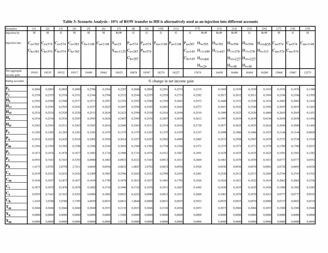
Using the model in Eq. (3), we have computed net aggregate and net sector-specific income effects under 19 scenarios given in Table 3. It should be notedthat the aggregate injection made under all these scenarios remains boundedby 10% of the RoW ′s transfers to four household groups. That is, in absoluteterms, the aggregate injection is equal to 1148 million Rwf. This would allowus to contrast the net effects of the RoW ′s direct transfers to households withthe effects implied by alternative policy interventions.Scenario [1], which represents the first best policy among the 19 scenarios,

reveals that investing in education and health generates the largest nationalincome gain. Assuming an exogenous investment in the education (Ce = 765)and health (Ch = 383) commodity sectors, this scenario leads to the maximumnet aggregate income gain of 19,545 mil Rwf. A comparison of net income gainsacross Scenarios [1], [2] and [4] demonstrate that a relatively higher investmentin education is welfare improving. Net aggregate income gain under Scenarios[2] and [4], which are respectively associated with the exogenous investmentpolicies of {Ce = Ch = 574} and {Ce = 383 < Ch = 765}, is smaller thanthat implied by Scenario [1]. Regarding the sectoral income effects, we find thata relatively higher investment in education paves the way for: (i) the H0, theH13 and Pa to absorb a significant portion of the income gains made and (ii) ahigher level of labor and capital employment relative to the employment froman equivalent investment in health.A comparison of Scenario [1] with [17] further demonstrates that investing in

education and health is not only welfare improving but also yields a higher levelof household income over the investment in the agricultural and manufacturingcommodity sectors.Under Scenario [2] and [3], an equal investment, Ce = Ch = 574, is made to

the education and health sectors separately through the savings-investment andthe government accounts. The investment made through the savings-investmentaccount is found to be more effi cient than the government investment. Thedifferences between the two scenarios are reflected in terms of higher capitaldemand (FC), income received by the H45 and demand for health production(Ph).When the whole amount of 1148 mil Rwf is invested only in the health sec-

tor, as assumed under Scenario [5], net aggregate income gain becomes smallerthan that under Scenarios [1]-[4]. This reveals that Scenario [5] is welfare re-ducing over Scenarios [1]-[4]. However, Scenario [5] is welfare improving overthe investment in either the agricultural or the manufacturing commodity sec-tors assumed under Scenarios [6]-[19]. This evidence lends a strong supportfor policies prioritizing higher investment in health relative to investment in theagricultural and the manufacturing sectors. The comparison of Scenario [5] with[6] also suggests that: (i) investing in health (agriculture) leads to higher growthof labor (capital) income relative to the investment in agriculture (health) and

12

(ii) investing in agriculture yields higher household income compared to the in-vestment in health, and households with more than 3 children (i.e., the H45 andthe H6) receive a larger proportion of this income. Consequently, agricultural(health) growth benefits large (small) families more.Do small families spend proportionally more on the education and health of

their children than large families? Scenarios [13] and [16] have been designedto answer this question. Under Scenario [13], only small families (i.e., the H0and the H13) experience an exogenous increase in their income, whereas underScenario [16], only large families (i.e., the H45 and the H6) experience the sameincrease. The estimations show that small families’demand for education andhealth commodities {Ce = 0.108, Ch = 0.094} under Scenario [13] is higherthan the demand by large families {Ce = 0.101, Ch = 0.090} under Scenario[16]. This finding proves that households with a small number of children investproportionally more on the education and health of their children than thosewith a large number of children.

3.3 Structural pathways and backward-forward linkages

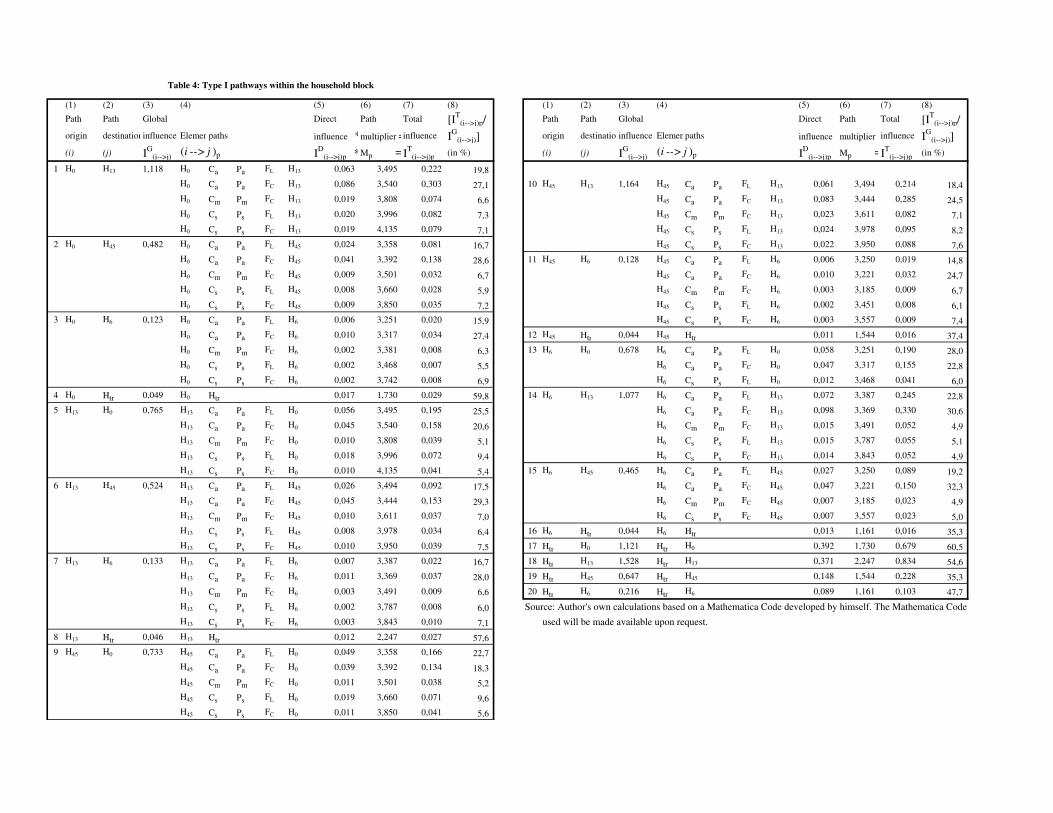
Four types of structural pathways are discussed using M ′.9 Type I pathwayscharacterize income transfers within the household block; Type II, the input-output multipliers within the production block; Type III, the multipliers ofeconomic influence of households on commodities; Type IV, the multipliers ofeconomic influence of production on factors; and Type V, the multipliers ofeconomic influence of exports on household income.Table 4 lists Type I pathways characterizing the effect of an exogenous

income transfer from one household group to another. For example, the globalinfluence of IG(H0 → H13) = mH0,H13

= 1.118 under Column 3 in Type I-1represents the multiplier effect on the H13 of an injection into the H0. That is,an injection of 100 Rwf into the H0 is expected to generate an additional incomeof 111.8 Rwf for the H13. Under Type I-1, five significant pathways account for68 % of the global influence.10 The most influential pathway from H0 to H13,{H0 → Ca → Pa → FC → H13}, accounts for 27.1 % of 111.8 Rwf. The otherpathways within the household block reveal that the global influence from H0 toH13 is exercised indirectly through intermediate accounts: {H0 → Ca → Pa →FL → H13} accounts for 19.8 % of the global influence; {H0 → Cs → Ps →FL → H13}, 7.3 % and so on. Likewise, under Column 3 in Type I-2, the globalinfluence of IG(H0 → H45) = mH0,H45

= 0.482 represents the multiplier effecton the H45 of an injection into the H0. Again, five significant pathways fromH0 to H45 explain 65 % of the global influence: {H0 → Ca → Pa → FC → H45}accounts for 28.6 % of the global influence; {H0 → Ca → Pa → FL → H45},16.7 %; {H0 → Cs → Ps → FC → H45}, 7.2 % and so on. Type I further shows

9Note that for notational convenience in this section we use M ′ (i.e., the transpose of M)and thus define mij as the multiplier effect from account i to account j.10A pathway is assumed to be significant if it transmits at least 5 % of the global influence

given in Column 8. Therefore, those pathways with less-than-five percent influence are notreported in tables.

13

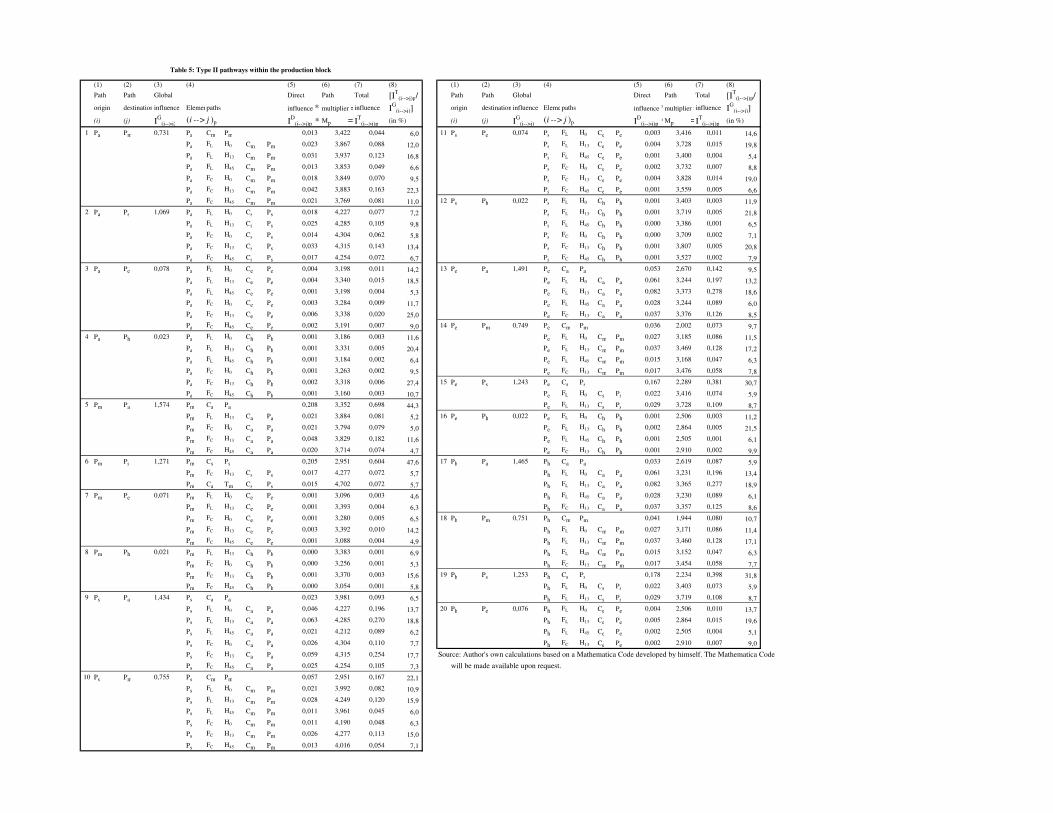
that indirect income transfers between any two household groups always takeplace through commodity, production and factors of production. In particular,agriculture plays the key role in facilitating significant income transfers betweenhouseholds. The main intermediate poles of income transfers include Ca, Pa, FLand FC , which clearly demonstrate the vitality of agriculture for promoting ruraldevelopment in Rwanda.Table 5 lists Type II pathways characterizing the interactions within the

production block. Feeding a very large number of people in Rwanda, agricul-ture and its linkages with the education and health sectors warrant a thoroughexamination because of the expected positive contribution to production of im-proved skill and health. Under Type II-3, only six pathways from agricultureto education account for 84 % of the global influence of mPa,Pe = 0.078. Themost important pathway, {Pa → FC → H13 → Ce → Pe}, accounts for 25 % ofthe global influence. This demonstrates that households with 1-3 children selltheir capital to the agricultural sector, and the factor income earned is spent oneducation, which in turn triggers the demand for the education services. Thesecond important pathway, {Pa → FL → H13 → Ce → Pe}, accounting for18,5 % of the global influence confirms the key role of the H13 in promotingeducation activities through labor income earned. In conclusion, 44 % of theglobal influence is determined by H13 as the key intermediate pole.Under Type II-4, again only six pathways from agricultural to health account

for 86 % of the global influence of mPa,Ph = 0.023. Of these, the most influentialpathways include {Pa → FC → H13 → Ch → Ph} and {Pa → FL → H13 →Ch → Ph} which respectively account for 27 % and 20 % of the global influence.Again, the H13 is the the most critical intermediate pole transmitting significantamount of economic influence from agriculture to health.Type II-13 shows the significant pathways from education to agriculture,

with a global influence of mPe,Pa = 1.49. Only five pathways explain 56 % ofthe global influence. The critical pathways, {Pe → FL → H13 → Ca → Pa} and{Pe → FL → H0 → Ca → Pa}, respectively account for 19 % and 13 % of theglobal influence. It should be noted that here households without children H0appears to be an important intermediate pole as well. Both H0 and H13 supplylabor (FL) and both spend the labor income earned on agricultural commodi-ties, which then stimulate agricultural production. This chain of interactionsdemonstrate that increasing demand for education boosts labor employment es-pecially among households with upto 3 children. Demand for capital appears toplay a limited role in agricultural production as well as employment creation,with a 9 % global influence.Type II-17 illustrates five significant pathways from health to agriculture,

explaing 53 % of the global influence mPh,Pa = 1.47. Two of these pathways,including {Ph → FL → H13 → Ca → Pa} and {Ph → FL → H0 → Ca → Pa},respectively account for 19 % and 13 % of the global influence. H0 and H13play an identical role as in Type II-13. It should be noted that about half of theglobal influence is explained by the pathways with less than 5 % explanatorypower. This shows that long-chain indirect effects are as important as theshorter pathways.

14

Three important findings evolve from a comparison of Type II-13 with TypeII-17. First of all, households up to 3 children play the key role in the transmis-sion of economic influence. Secondly, investment in the education and healthsectors boosts substantial employment of labor. Lastly, the promotion of educa-tion and health production is likely to give a momentum not only to agriculturalbut also to manufacturing and service sectors, which is implied by very largeincome multipliers of an injection into the health and education sectors.The significant pathways listed under Type II-16 and II-20 help understand

the nature of interaction between the two public services. Type II-16 declaresfour important pathways from education to health, explaining almost half of theglobal influencemPe,Ph = 0.022. The pathways, {Pe → FL → H13 → Ch → Ph}and {Pe → FL → H0 → Ch → Ph}, respectively explain 22 % and 11 % of theglobal influence. With a 10 % explanatory power, the pathway {Pe → FC →H13 → Ch → Ph} occupies the third place in ranking. H0 and H13 play arole comparable the pathways discussed in the previous paragraph. Type II-20also declare four critical pathways from health to education, explaining abouthalf of the global influence mPh,Pe = 0.076. Again, households with up to threechildren play a dominant role in the transmission of the influence from healthto education. Interestingly, mPh,Pe = 0.076 > mPe,Ph = 0.022 reveals that theinfluence of health on education is about four times stronger than that of theeducation on health.Table 6 lists Type III pathways characterizing the impact of an exogenous

increase in household income on commodity demand. The focus is in particularon the impact on the demand for the education and health commodities, whichconcern the pathways under Type III-4, III-5, III-10, III-11, III-16, III-17, III-22,III-23, III-28 and III-29. With respect to the effect on education, H13 occupiesthe first place with a global influence of mH13,Ce = 0.087 under Type III-10.Sixty-four percent of this global influence is accounted for only by a single,direct path from H13 to Ce. Next comes H0 with mH0,Ce = 0.081 under TypeIII-4, which accounts for 53 % of the global influence. It is also important tonote that, under Type III-28, H13 acts as the key intermediate pole effectivelytransmitting income from Htr to Ce, explaining 25 % of mHtr,Ce = 0.083. H0occupies the second place, accounting for 21 % of mHtr,Ce = 0.083. Concerningthe health effects under Type III-5, III-11, III-17, III-23 and III-29, householdgroups are ranked in the same order as above but the multipliers associatedwith them are much smaller than those in the case of education. A commonobservation among the education and health pathways discussed so far is thatlonger chain pathways with less than 5 % explanatory power also play a criticalrole in promoting the demand for human capital.Table 7 shows Type IV pathways characterizing the impact on factor de-

mand of an exogenous increase in production. A comparison of the productionmultipliers across labor and capital inputs given in (MFP

2,5 )′ (i.e., compare the

figures in the1st with those in the 2nd column of (MFP2,5 )

′) demonstrates thatthe agricultural, manufacturing and service sectors (the education and healthsectors) promote higher capital (labor) employment than labor (capital) em-

15

ployment when the demand equally rises for these production activities. Direct,binary paths in Table 7 explain a very large share of the global influence, includ-ing {Pa → FC explains 85 % of the global influence; Ps → FC , 65 %; Pm → FC ,44 %; Pe → FL, 63 % and Ph → FL, 63 %}. The corresponding path multipliersgiven in Column (6) further imply that these one-edge paths are substantiallyinfluenced by loops around the path origin. To sum up, increasing demand forhuman capital would create proportionally higher labor employment.Table 8 shows Type V pathways characterizing the impact on household

income of an exogenous increase in the export demand. The exports of Rwandainclude agricultural and manufacturing goods only. Regarding the impact ofagricultural exports, H13 obtains the largest income gain with an income multi-plier of 1.542: one unit increase in agricultural exports generates 1.542 units ofincome for households with 1-3 children. Fifty-one percent of 1.542 is explainedby capital demand from H13, whereas 38 percent is explained by labor demandfrom H13. With an income multiplier of 0.966, H0 follows H13. Labor supply ofH0 explains 47 % of the income multiplier, while capital supply explains 38 %.These findings confirm that, in absolute terms, H13 dominates over H0 in termsof labor as well as capital income multiplier effects created by unit rise in exportdemand. (The same result also holds for the manufacturing export sector.) Inconclusion, increasing exports would benefit households with 1-3 children themost, followed by households with no children.Backward (or diffusion) and forward (or absorption) linkage analysis helps

us identify the "key" sectors of the Rwandan economy. A sector is called "key"if it leads to an over-average impact on the whole economy either through anexogenous change in its own demand structure or through a change in its demandstructure induced by the rest of the economy. To identify the key sectors,the Multiplier Product Matrix (MPM) and the backward and forward linkageindices are calculated as follows:

MPM = [mpmij ]i,j=1,...,n =| mi· m·j |

m

bj =m·j(m/n)

, j = 1, 2, ..., n "backward linkages"

fi =mi·(m/n)

, i = 1, 2, ..., n "forward linkages"

where m =

n=21∑i=1

n=21∑j=1

mij = sum of all the multipliers in M

mi· = sum of the multipliers in row i of M

m·j = sum of the multipliers in column j of M

| mi· m·j |= absolute value of the product mi· and m·j

Table 9 shows that, with fCa = 219 %, the agricultural commodity sector hasthe highest forward linkage. This means that a unit change in the demandof the rest of the economy affects agriculture the most, with a 119 % higherthan the economy-wide average multiplier. Other sectors significantly affected

16

by changes in the rest of the economic system include capital and agriculturaloutput with a 117 % higher than the economy-wide average multiplier impliedby fFC , fPa = 217 %, the manufacturing commodity sector with a 104 %higher multiplier from fCm = 204 %, labor with a 95 % higher multiplier fromfFL = 195 % and the H13 with a 94 % higher multiplier from fH13

= 194 % andso on.On the other hand, with bTm = 117 %, trade margin has the highest back-

ward linkage. This means that a unit exogenous increase in trade margin wouldyield 17 % higher economic activity in the rest of the economy than that im-plied by the economy-wide average multiplier. With bCe = 115 %, the educationcommodity sector occupies the 2nd place; that is, a unit exogenous increase inthe demand of education would yield a 15 % higher activity level than thatimplied by the average multiplier. The health commodity sector as well as theagricultural and manufacturing export sectors all together take the 3rd place;that is, a unit increase in the demand of these sectors would separately promote14 % more economic activity than that implied by the average multiplier.Three important findings are in order. First, implied by their significant

backward linkages, Ce and Ch tend to transmit their growth to the rest of theeconomy more effectively than others. Second, H13 is able to internalize moreeffectively the growth that other sectors of the economy experience. Lastly,Ce, Ch, Pe, Ph, and Xa and Xm seem to perform poorly in absorbing thegrowth effects taking place in the rest of the economy.

4 Discussion

MULTIPLIER ANALYSIS confirms that family size is an important factor inthe formation of human capital. In the context of Rwanda, households with 1-3children, which is less than the national average family size of 5, tend to investin the education and health of their children significantly more than householdswith 4 or more children. This suggests that the 2006 SAM of Rwanda representsan economy in which family size is inversly related to human capital investment.Implementing family planning programs thus seems to be a viable option for thepromotion of human capital-based economic development.With respect to poverty reduction, the results further confirm that house-

holds with small family size perform a leading role in the economy-wide incomegeneration and experience the largest income gain from an investment in humancapital. Given an income stimulus for the education and health production,households with upto 3 children experience the highest income gain. Exportgrowth also favors the same households in terms of income growth.As to household income transfers, the results demonstrate that households

with 1-3 children tend to receive more indirect transfers than the transfers itactually makes to others. Due to the absence of direct income transfers acrosshouseholds, all the transfers represented by the multipliers within the house-hold block stand for the rate of indirect household transfers resulting from theeconomic interactions between households. Income distribution pattern show

17

that increasing demand for human capital rises labor demand accomodated ata higher rate by the labor supply of households with 1-3 children. On the otherhand, higher employment of capital takes place in agriculture, manufacture andservices, which benefits households with 4-5 children the most.SCENARIO ANALYSIS reveals that, in terms of net aggregate income gain,

human capital investment is the first-best policy in Rwanda relative to invest-ment in agriculture, manufacturing and service sectors. Specifically, with a largeemployment multiplier effect, education and health investment benefits small-size families the most. Within the SAM framework, such an investment can bechanneled through either the S-I account or the government account. The sce-narios carried out support the hypothesis that investment funds released fromthe S-I account do the job more effi ciently than those from the government ac-count. These findings suggest that in the context of Rwanda policies should givepriority to human capital investment because small families contribute directlyto increasing the human capital of children; higher fertility impedes humancapital formation, for given resources. Dissemination of information to familiesabout the negative consequences of high fertility for their children and providingthe means for controlling fertility should be high priorities for public agencies.In terms of net aggregate income gain, large families benefit more from agri-

cultural growth, while small families benefit more from human capital growth.Furthermore, small families demand human capital commodities more than largefamilies. Together, These findings confirm the assertion that households witha smaller number of children tend to invest marginally more on the educationand health of their children than those with a larger number of children.PATH ANALYSIS shows that households interact with each other only

through elementary pathways from commodities, to production activities and tofactors. There is no direct binary path among household groups. Regarding theintersectoral influence, the most important pathway, {Pa → FC → H13 → Ce →Pe}, clearly shows that the H13 finances its demand for education commoditythrough its capital income from the agricultural sector. The secondary sourceof H13’s education expenditure is its labor income. Together, the capital andlabor income of H13 accounts for about half of the global influence on educationof a unite increase in agricultural production. Regarding the health commoditydemand, we observe the same pattern in which H13 is the most critical interme-diate pole. To sum up, H13 has more savings (or capital) than other householdsand invests more in the education and health of their children.An improvement in human capital (i.e., education and health) is expected to

have an important impact on agricultural production through the enhancementof allocative effi ciency. The path analysis suggests that there is ample scope forincreasing investment in human capital to promote agricultural production. Onecould easily see that if the government of Rwanda aims to promote agriculturalsector, the investment in education and health should occupy the top of its policyagenda. Agaian, the H13 seems to be the key intermediate pole in transmittingthe influence of such an investment to agriculture in particular and to the restof the economy in general.The linkage analysis shows that the agricultural commodity sector is the key

18

sector in the Rwandan economy, followed by the education and health commod-ity sectors. Furthermore, the education and health sectors promote significantgrowth in other sectors of the economy and act as the engine of growth in theagriculture, manufacturing and service sectors. The household group with thehighest allocative effi ciency remains to be the H13 as it is the group which caneffectively internalize economic growth.

5 Summary and Conclusions

The main purpose of this paper is to explore the role of different householdgroups in the formation of human capital, employment, sectoral growth and in-come distribution in Rwanda. The 2006 SAM used in the analysis represents ageneral equilibrium data system of the Rwandan economy. The multiplier andstructural path analyses are applied to examine the transmission of economicinfluences across institutions. The paper first computes income multipliers tocharacterize the macroeconomic transmission of economic influences stimulatedby an exogenous increase in demand. Then, applying the SPA, it identifies thecritical, individual transmission pathways behind these computed income mul-tipliers and explores macroeconomic effects of different groups of households onhuman capital formation, employment, sectoral growth and income distribution.The following two findings are noted. First, the smaller the number of chil-

dren in an average family, the higher the investment in human capital of thechildren in that family, demonstrating the presence of quantity-quality trade-off.In particular, the household group with 1-3 children tends to spend more for theimprovement of education and health status of children than those householdgroups with more than 3 children. Second, an improvement in human capitalleads to a significant increase in agricultural production and that householdswith 1-3 children act as an important intermediate pole transmitting the in-fluence of human capital investment on agricultural production. In conclusion,promoting family planning programs in Rwanda thus seems to be a viable strat-egy for economic growth and poverty reduction, considering the current averagefamily size of 5 children.Some final remarks should be made on the limitation of the current study.

First, the SAM data framework assumes that expenditure of an account rep-resents the influece of that account on other accounts. In reality, the actualinfluence of one account on other accounts can be better approximated througha more detailed econometric causality estimation between the relevant accounts.Second, the multiplier analysis draws on average expenditure propensities ob-tained from the SAM, while marginal propensities are more reliable to depictnon-linear structural relations. In other words, the implicit assumption of uni-tary expenditure elasticities may not reflect the actual behaviour of an insti-tution and hence the SAM multiplier analysis may deviate from the realitieson the ground. Third, disaggregation of the SAM accounts is arbitrary. Forexample, that agriculture is represented as a single account in the SAM implic-itly assumes that all farm types produce an identical output mix using the same

19

technology. This makes the estimated results conditional on the type and natureof policies analysed. Given the issues analyzed in this work, the highly disag-gregated representation of health and education accounts would not add muchto the analysis of economy-wide effects of human capital investment. Fourth,the SAM multiplier method is limited in its ability to provide a picture of thefeedback interactions between the sectors of an economy because a SAM givesonly a snopshot picture of the transactions in a given year. The feedback analy-sis obviously demands for a time-series of SAMs but the construction of sucha time series is very rare in practice. CGE models have largely overcome thislimitation, allowing to investigate the economy-wide growth and distributiveoutcomes of exogenous changes in market conditions or policies simultaneouslyimplemented. Last but not least, the SAM multiplier method cannot be appliedif income changes follow a stochastic process. Methodological advancement isneeded to analyze stochastic income multiplier effects.All together, these limitations may justify the development of two modeling

frameworks. The CGE modelling framework is generally considered as a nat-ural extension of a SAM-based multiplier model. Even if referring to differenttheoretical frameworks, studies in the literature generally agree that these twomodels yield complementary results to policy analysis. Finally, a more signif-icant improvement in modelling the economy-wide effects of households couldprobably be obtained by developing an integrated micro—macro approach. Theavailability of a suitable database would allow researchers to build a micro-simulation model of households, and to link it to the macro-economic frameworkthrough the SAM.

20

References

[1] Angrist, Joshua D., Victor Lavy, and Analia Schlosser. 2005. "New Ev-idence on the Causal Link Between the Quantity and Quality of Chil-dren." National Bureau of Economic Research Working Paper 11835.http://www.nber.org/papers/w11835

[2] Ansoms, An. (2008). "A Green Revolution for Rwanda? The Political Econ-omy of Poverty and Agrarian Change." Institute of Development Policy andManagement Discussion Paper 2008-06.

[3] Azarnert, Leonid V. 2004. "Redistribution, Fertility and Growth: the Effectof the Opportunities Abroad." European Economic Review, 48: 785-795.

[4] Barro, Robert J., and Gery S. Becker. 1989. "Fertility choice in a Model ofEconomic Growth." Econometrica, 57: 481-502.

[5] Becker, Gery S., and Robert J. Barro. 1988. "A Reformulation of the Eco-nomic Theory of Fertility." Quarterly Journal of Economics, 53(1): 1-25.

[6] Becker, Gery S., Kevin M. Murphy, Robert F. Tamura. 1990. "HumanCapital, Fertility and Economic Growth." Journal of Political Economy,98: 12-37.

[7] Benhabib, Jess., and Mark M. Spiegel. 1994. "The Role of Human Capitalin Economic Development: Evidence from Aggregate Cross-country Data."Journal of Monetary Economics, 34: 143-173.

[8] Bigsten, Arne, and Ann-Sofie Isaksson. 2008. “Growth and Povertyin Rwanda: Evaluating the EDPRS 2008-12.” Swedish Interna-tional Development Cooperation Agency Country Economic Report 3.http://www.hgu.gu.se/Files/nationalekonomi/Personal/Isaksson%20Ann-Sofie/SIDA%20report%202008.pdf.

[9] Bloom, David, David Canning, and Jaypee Sevilla. 2001. “EconomicGrowth and the Demographic Transition.”NBER Working Paper 8685.

[10] – – – -. 2003. "The Effect of Health on Economic Growth: a ProductionFrontier Approach." World Development, 32(1): 1-13.

[11] Defourny, J., and Thorbecke, E. (1984). Structural path analysis and multi-plier decomposition within a SAM Framework. Economic Journal, 94 (373),111-136.

[12] Diao, Xinshen, Shenggen Fan, Sam Kanyarukiga, and Bingxin Yu. 2010.Agricultural Growth and Investment Options for Poverty Reduction inRwanda. Washington, D.C., USA: IFPRI (International Food Policy Re-search Institute). Research Monograph.

[13] Emini, Christian A. 2007. “The 2006 Social Accounting Matrix of Rwanda:Methodology Note." Unpublished.

21

[14] Hossain, Shaikh. 1989. "Effect of Public Programs on Family Size, ChildEducation and Health." Journal of Development Economics, 30: 145-158.

[15] Joshi, Shareen, and T. Paul Schultz. 2007. "Family Planning as an In-vestment in Development: Evaluation of a Program’s Consequences inMatlab, Bangladesh." Economic Growth Center Discussion Paper 951.http://www.econ.yale.edu/~egcenter/

[16] Khan, Abrahim H., and Erik Thorbecke. 1989. “Macroeconomic Effects ofTechnological Change: Multiplier and Structural Path Analysis within aSAM Framework.”Journal of Policy Modeling, 11(1): 131-156.

[17] MINECOFIN (Ministry of Finance and Economic Planning). 2007. “Eco-nomic Development and Poverty Reduction Strategy: 2008-2012.”Kigali,Rwanda: MINECOFIN, Republic of Rwanda.

[18] Oded, Galor, and David N. Weil. 1996. "The Gender Gap, Fertility andGrowth." American Economic Review, 86: 374-387.

[19] – – – -. 2000. "Population, Technology, and Growth: from the Malthu-sian Stagnation to the Demographic Transition and Beyond." AmericanEconomic Review, 90: 806-828.

[20] Osorio, Parra, Juan Carlos and Wodon Quentin. 2010. "How Does GrowthAffect Labor Income by Gender? A Structural Path Analysis for Tanzania."University Library of Munich MPRA Paper 27735. http://mpra.ub.uni-muenchen.de/27735/

[21] Pyatt, Graham, and Jeffery I. Round. 1985. Social Accounting: A Basis forPlaning. World Bank and Oxford University Press.

[22] Roberts, Deborah. (1996). "UK Agriculture in the Wider Economy: theImportance of Net SAM Linkage Effects. European Review of AgriculturalEconomics, 22: 495-454.

[23] – – – -. 2005. “The Role of Households in Sustaining Rural Economies:A Structural Path Analysis.”European Review of Agricultural Economics,32(3): 393-420.

[24] Roland-Host, David W., and Ferran Sancho. 1992. “Relative Income Deter-mination in the United States: A Social Accounting Perspective.”Reviewof Income and Wealth, 38(3): 311-27.

[25] Rosenzweig, Mark R. 1988. “Human Capital, Population Growth and Eco-nomic Development: Beyond Correlations.” Journal of Policy Modeling,10(1): 83-111.

[26] Rosenzweig, Mark R., and Kenneth I. Wolpin. 1986. "Evaluating the Ef-fects of Optimally Distributed Public Programs: Child Health and FamilyPlanning Interventions." American Economic Review, 76(3): 470-482.

22

[27] Rosenzweig, Mark R., and Junsen Zhang. 2009. "Do Population ControlPolicies Induce More Human Capital Investment? Twins, Birth Weight andChina’s “One-Child” Policy." Review of Economic Studies, 76(3): 1149-1174.

[28] Ross, John A., W. Parker Mauldin, Steven R. Green, and E. RomanaCooke. 1992. Family Planning and Child Survival Programs as Assessed in1991. New York: Population Council.

[29] Round, Jeffery I. 2003. Social accounting matrices and SAM-based multi-plier analysis. In Francois Bourguignon and Luiz A. Pereira da Silva (Eds.),The impact of economic policies on poverty and income distribution: Eval-uation techniques and tools. New York: Oxford University Press for theWorld Bank.

[30] Schultz, T. Paul. 2005. “Effects of Fertility Decline on Family Well-Being:Evaluation of Population Programs.” Paper presented at the MacArthurFoundation Consultation meeting, Philadelphia, PA.

[31] – – – -. 1997. "Diminishing Returns to Scale in Fam-ily Planning Expenditures, Thailand, 1976-1981."http://www.econ.yale.edu/~pschultz/thai.pdf

[32] Schütt, Florian. 2003. "The Importance of Human Capital for EconomicGrowth." Institut für Weltwirtschaft und Internationales Management Uni-versität Bremen Working Paper 27.

[33] Solo, Julie. 2008. Family Planning in Rwanda: How a Taboo Topic BecamePriority Number One. Chapel Hill, NC, USA: IntraHealth.

[34] Thorbecke, Erik. 1995. Intersectoral Linkages and their Impact on RuralPoverty Alleviation: A SAM. Vienna, Republic of Austria: UNIDO.

[35] Thorbecke, Erik., and Hong-Sang Jung. 1996. "A Multiplier Decompo-sition Method to Analyze Poverty Alleviation." Journal of DevelopmentEconomics, 48: 279-300.

[36] Whalley, John, and France St-Hillaire. 1987. “A Microconsistent Data Setfor Canada for Use in Regional General Equilibrium Policy Analysis.”Re-view of Income and Wealth, 33: 327-343.

[37] World Bank. 1990. World Development Report. Oxford: Oxford UniversityPress.

23

FL FC H0 H13 H45 H6 Htr Fr Pa Pm Ps Pe Ph Ca Cm Cs Ce Ch Tm Xa Xm G SI RoW

FL 0 0 0 0 0 0 0 0 287755 67320 285603 43449 14118 0 0 0 0 0 0 0 0 0 0 0

FC 0 0 0 0 0 0 0 0 367715 144915 252057 18607 6046 0 0 0 0 0 0 0 0 0 0 0

H0 241788 170769 0 0 0 0 7502 0 0 0 0 0 0 0 0 0 0 0 0 0 0 0 0 5937

H13 299924 358471 0 0 0 0 7090 0 0 0 0 0 0 0 0 0 0 0 0 0 0 0 0 3783

H45 113472 170493 0 0 0 0 2827 0 0 0 0 0 0 0 0 0 0 0 0 0 0 0 0 1271

H6 28461 42483 0 0 0 0 1698 0 0 0 0 0 0 0 0 0 0 0 0 0 0 0 0 477

Htr 0 0 7145 7931 3062 978 0 0 0 0 0 0 0 0 0 0 0 0 0 0 0 0 0 0

Fr 0 47124 0 0 0 0 0 0 0 0 0 0 0 0 0 0 0 0 0 0 0 8569 0 30839

Pa 0 0 0 0 0 0 0 0 0 0 0 0 0 697883 0 0 0 0 0 1485 0 0 0 0

Pm 0 0 0 0 0 0 0 0 0 0 0 0 0 0 468471 0 0 0 0 0 74340 0 0 0

Ps 0 0 0 0 0 0 0 0 0 0 0 0 0 0 0 763470 0 0 0 0 0 0 0 0

Pe 0 0 0 0 0 0 0 0 0 0 0 0 0 0 0 0 88812 0 0 0 0 0 0 0

Ph 0 0 0 0 0 0 0 0 0 0 0 0 0 0 0 0 0 28857 0 0 0 0 0 0

Ca 0 0 164586 282874 107673 32295 0 0 17599 121740 19216 5089 1029 0 0 0 0 0 0 0 0 0 0 0

Cm 0 0 136554 237483 109199 18242 0 0 18089 95007 86944 6511 2396 0 0 0 0 0 0 0 0 0 233582 0

Cs 0 0 55433 95050 43902 6807 0 0 8210 113830 119650 15155 5268 0 0 0 0 0 150020 0 0 168479 0 0

Ce 0 0 10442 16482 5589 1650 0 0 0 0 0 0 0 0 0 0 0 0 0 0 0 54649 0 0

Ch 0 0 2504 5379 1985 187 0 0 0 0 0 0 0 0 0 0 0 0 0 0 0 18818 0 0

Tm 0 0 0 0 0 0 0 0 0 0 0 0 0 52682 97338 0 0 0 0 0 0 0 0 0

Xa 0 0 0 0 0 0 0 0 0 0 0 0 0 0 0 0 0 0 0 0 0 0 0 1485

Xm 0 0 0 0 0 0 0 0 0 0 0 0 0 0 0 0 0 0 0 0 0 0 0 74340

G 0 0 19405 11652 4054 539 0 28766 0 0 0 0 0 105 110412 18334 0 17 0 0 0 193283 0 168673

SI 0 0 27909 10088 11981 12319 0 38699 0 0 0 0 0 0 0 0 0 0 0 0 0 -2258 0 134844

RoW 14600 0 2019 2328 617 103 0 19068 0 0 0 0 0 1431 267786 0 0 0 0 0 0 113699 0 0

Endogenous Accounts Exogenous Accounts

Table 1: Social Accounting Matrix for Rwanda, 2006

FL FC H0 H13 H45 H6 Htr Fr Pa Pm Ps Pe Ph Ca Cm Cs Ce Ch Tm Xa Xm

FL 2,17 1,13 1,14 1,24 1,19 1,10 1,18 0,00 1,57 1,39 1,56 1,71 1,70 1,56 0,85 1,52 1,71 1,70 1,52 1,57 1,39

FC 1,37 2,32 1,34 1,46 1,40 1,29 1,39 0,00 1,88 1,74 1,71 1,62 1,61 1,86 1,03 1,67 1,62 1,61 1,67 1,88 1,74

H0 1,07 0,91 1,70 0,77 0,73 0,68 1,12 0,00 0,97 0,87 0,93 0,96 0,96 0,96 0,53 0,90 0,96 0,95 0,90 0,97 0,87

H13 1,57 1,56 1,12 2,21 1,16 1,08 1,53 0,00 1,54 1,40 1,46 1,49 1,48 1,53 0,84 1,43 1,49 1,48 1,43 1,54 1,40

H45 0,66 0,69 0,48 0,52 1,50 0,46 0,65 0,00 0,67 0,61 0,63 0,63 0,63 0,66 0,36 0,61 0,63 0,63 0,61 0,67 0,61

H6 0,17 0,18 0,12 0,13 0,13 1,12 0,22 0,00 0,17 0,15 0,16 0,16 0,16 0,17 0,09 0,16 0,16 0,16 0,16 0,17 0,15

Htr 0,05 0,04 0,05 0,05 0,04 0,04 1,05 0,00 0,04 0,04 0,04 0,04 0,04 0,04 0,02 0,04 0,04 0,04 0,04 0,04 0,04

Fr 0,08 0,14 0,08 0,09 0,08 0,08 0,08 1,00 0,11 0,10 0,10 0,10 0,10 0,11 0,06 0,10 0,10 0,10 0,10 0,11 0,10

Pa 1,51 1,46 1,48 1,61 1,52 1,48 1,54 0,00 2,49 1,57 1,43 1,49 1,46 2,41 0,93 1,40 1,49 1,46 1,40 2,49 1,57

Pm 0,74 0,71 0,72 0,78 0,77 0,66 0,75 0,00 0,73 1,77 0,75 0,75 0,75 0,73 0,95 0,74 0,75 0,75 0,74 0,73 1,77

Ps 1,08 1,04 1,05 1,15 1,12 0,96 1,09 0,00 1,07 1,27 2,21 1,24 1,25 1,14 0,85 2,16 1,24 1,25 2,16 1,07 1,27

Pe 0,08 0,08 0,08 0,09 0,08 0,08 0,08 0,00 0,08 0,07 0,07 1,08 0,08 0,08 0,04 0,07 1,08 0,08 0,07 0,08 0,07

Ph 0,02 0,02 0,02 0,03 0,02 0,02 0,02 0,00 0,02 0,02 0,02 0,02 1,02 0,02 0,01 0,02 0,02 1,02 0,02 0,02 0,02

Ca 1,63 1,57 1,60 1,74 1,64 1,60 1,66 0,00 1,61 1,70 1,55 1,61 1,58 2,60 1,00 1,51 1,61 1,58 1,51 1,61 1,70

Cm 1,49 1,44 1,45 1,58 1,56 1,33 1,50 0,00 1,47 1,55 1,52 1,51 1,51 1,47 1,92 1,48 1,51 1,51 1,48 1,47 1,55

Cs 1,10 1,07 1,08 1,17 1,15 0,99 1,12 0,00 1,09 1,30 1,24 1,27 1,28 1,17 0,87 2,21 1,27 1,28 2,21 1,09 1,30

Ce 0,08 0,08 0,08 0,09 0,08 0,08 0,08 0,00 0,08 0,07 0,07 0,08 0,08 0,08 0,04 0,07 1,08 0,08 0,07 0,08 0,07

Ch 0,02 0,02 0,02 0,03 0,02 0,02 0,02 0,00 0,02 0,02 0,02 0,02 0,02 0,02 0,01 0,02 0,02 1,02 0,02 0,02 0,02

Tm 0,27 0,26 0,26 0,28 0,28 0,25 0,27 0,00 0,26 0,28 0,27 0,27 0,27 0,33 0,27 0,26 0,27 0,27 1,26 0,26 0,28

Xa 0,00 0,00 0,00 0,00 0,00 0,00 0,00 0,00 0,00 0,00 0,00 0,00 0,00 0,00 0,00 0,00 0,00 0,00 0,00 1,00 0,00

Xm 0,00 0,00 0,00 0,00 0,00 0,00 0,00 0,00 0,00 0,00 0,00 0,00 0,00 0,00 0,00 0,00 0,00 0,00 0,00 0,00 1,00

Table 2: Global Multiplier Matrix M

Scenarios [1] [2] [3] [4] [5] [6] [7] [8] [9] [10] [11] [13] [14] [15] [16] [17] [18] [19]

Injection by SI SI G SI SI SI RoW G G G G G RoW RoW RoW G RoW SI G SI

Injection into Ce=765 Ce=574 Ce=574 Ce=383 Ch=1148 Ca=1148 Xa=23 Pa=574 Pe=574 Pm=1148 Pa=1148 Pa=287 H0=295 H0=701 H0=594 H0=594 H45=835 Ca=574 Ca=574 Cm=1148

Ch=383 Ch=574 Ch=574 Ch=765 Xm=1125 Ce=287 Ph=574 Ce=145 H13=189 H13=447 H13=378 H13=378 H6=313 Cm=574 Cm=574

Ch=287 Ch=145 H45=64 H45=127 H45=127

H6=24 H6=48 H6=48

Net aggregate

income gain

FL 0,2804 0,2803 0,2803 0,2800 0,2796 0,2564 0,2287 0,2688 0,2804 0,2281 0,2574 0,1945 0,1939 0,1939 0,1919 0,1976 0,1976 0,1389

FC 0,2358 0,2355 0,2354 0,2351 0,2346 0,2706 0,2532 0,2544 0,2355 0,2529 0,2733 0,2017 0,2012 0,2011 0,1994 0,2106 0,2106 0,1505

H0 0,2582 0,2580 0,2580 0,2577 0,2573 0,2587 0,2354 0,2592 0,2580 0,2350 0,2603 0,3608 0,3352 0,3350 0,1934 0,2002 0,2002 0,1418

H13 0,2546 0,2545 0,2545 0,2542 0,2537 0,2625 0,2407 0,2594 0,2545 0,2401 0,2645 0,2651 0,2542 0,2540 0,1956 0,2035 0,2035 0,1443

H45 0,2524 0,2524 0,2520 0,2520 0,2513 0,2638 0,2423 0,2590 0,2520 0,2416 0,2656 0,1989 0,2423 0,2420 0,4860 0,2045 0,2045 0,1451

H6 0,2516 0,2516 0,2516 0,2503 0,2503 0,2626 0,2407 0,2585 0,2516 0,2407 0,2639 0,1997 0,2639 0,2639 0,6236 0,2038 0,2038 0,1436

Htr 0,2563 0,2563 0,2511 0,2563 0,2563 0,2616 0,2406 0,2563 0,2511 0,2354 0,2616 0,2877 0,2825 0,2825 0,2616 0,2040 0,2040 0,1465

Fr 0,1283 0,1283 0,1283 0,1283 0,1283 0,1479 0,1375 0,1375 0,1283 0,1375 0,1479 0,1098 0,1086 0,1086 0,1075 0,1144 0,1144 0,0820

Pa 0,2432 0,2425 0,2425 0,2418 0,2402 0,3956 0,2614 0,3257 0,2425 0,2582 0,4089 0,2515 0,2508 0,2507 0,2479 0,2737 0,2738 0,1519

Pm 0,1584 0,1584 0,1584 0,1586 0,1586 0,1544 0,3694 0,1566 0,1584 0,3738 0,1546 0,1575 0,1573 0,1571 0,1570 0,1780 0,1780 0,2015

Ps 0,1873 0,1876 0,1876 0,1877 0,1882 0,1718 0,1906 0,1741 0,1876 0,1911 0,1607 0,1639 0,1635 0,1635 0,1625 0,1501 0,1501 0,1282

Pe 0,9593 0,7443 0,7443 0,5292 0,0980 0,1002 0,0923 0,4222 0,7443 0,0912 0,1013 0,1081 0,1070 0,1070 0,1013 0,0777 0,0777 0,0552

Ph 1,4173 2,0792 2,0758 2,7411 4,0649 0,0936 0,0832 1,0847 2,0792 0,0832 0,0936 0,0936 0,0936 0,0970 0,0901 0,0728 0,0693 0,0520

Ca 0,2439 0,2432 0,2432 0,2424 0,2409 0,3965 0,2586 0,2442 0,2432 0,2590 0,2454 0,2520 0,2512 0,2513 0,2484 0,2744 0,2743 0,1522

Cm 0,1836 0,1837 0,1837 0,1837 0,1839 0,1789 0,1878 0,1815 0,1837 0,1881 0,1792 0,1824 0,1821 0,1822 0,1819 0,2062 0,2062 0,2336

Cs 0,1873 0,1875 0,1876 0,1878 0,1882 0,1718 0,1906 0,1742 0,1876 0,1911 0,1607 0,1639 0,1635 0,1635 0,1626 0,1500 0,1502 0,1283

Ce 0,9593 0,7443 0,7443 0,5292 0,0980 0,1002 0,0923 0,4222 0,0980 0,0912 0,1013 0,1081 0,1070 0,1070 0,1013 0,0777 0,0777 0,0552

Ch 1,4165 2,0780 2,0780 2,7395 4,0659 0,0935 0,0831 1,0840 0,0900 0,0831 0,0935 0,0935 0,0935 0,0970 0,0900 0,0727 0,0693 0,0519

Tm 0,2046 0,2046 0,2046 0,2040 0,2040 0,2553 0,2133 0,2033 0,2046 0,2126 0,2026 0,2073 0,2066 0,2066 0,2053 0,2300 0,2300 0,2046

Xa 0,0000 0,0000 0,0000 0,0000 0,0000 0,0000 1,5488 0,0000 0,0000 0,0000 0,0000 0,0000 0,0000 0,0000 0,0000 0,0000 0,0000 0,0000

Xm 0,0000 0,0000 0,0000 0,0000 0,0000 0,0000 1,5133 0,0000 0,0000 0,0000 0,0000 0,0000 0,0000 0,0000 0,0000 0,0000 0,0000 0,0000

Table 3: Scenario Analysis - 10% of ROW transfer to HH is alternatively used as an injection into different accounts

[12]

19545 19535 19532 19517 19489 19461 19425

Endog accounts % change in net income gain

0,2319

17674 16450 16406 1640418274 18227 1586718878 18387

0,1691

0,2669

0,2885

0,1571

0,1820

16269

0,2573

0,2282

0,2972

0,0000

0,1692

12273

0,5926

0,2481

15868

0,2510

0,2612

0,2720

0,1237

0,2669

0,5922

0,2053

0,0000

(1) (2) (3) (4) (5) (6) (7) (8) (1) (2) (3) (4) (5) (6) (7) (8)

Path Path Global Direct Path Total [IT

(i-->j)p/ Path Path Global Direct Path Total [IT

(i-->j)p/

origin destinationinfluence Elementarypaths influence *multiplier =influence IG

(i-->j)] origin destinationinfluence Elementarypaths influence multiplier =influence IG

(i-->j)]

(i) (j) IG

(i-->j) ID

(i-->j)p *Mp = IT

(i-->j)p(in %) (i) (j) I

G(i-->j) I

D(i-->j)p

Mp =IT

(i-->j)p(in %)

1 H0 H13 1,118 H0 Ca Pa FL H13 0,063 3,495 0,222 19,8

H0 Ca Pa FC H13 0,086 3,540 0,303 27,1 10 H45 H13 1,164 H45 Ca Pa FL H13 0,061 3,494 0,214 18,4

H0 Cm Pm FC H13 0,019 3,808 0,074 6,6 H45 Ca Pa FC H13 0,083 3,444 0,285 24,5

H0 Cs Ps FL H13 0,020 3,996 0,082 7,3 H45 Cm Pm FC H13 0,023 3,611 0,082 7,1

H0 Cs Ps FC H13 0,019 4,135 0,079 7,1 H45 Cs Ps FL H13 0,024 3,978 0,095 8,2

2 H0 H45 0,482 H0 Ca Pa FL H45 0,024 3,358 0,081 16,7 H45 Cs Ps FC H13 0,022 3,950 0,088 7,6

H0 Ca Pa FC H45 0,041 3,392 0,138 28,6 11 H45 H6 0,128 H45 Ca Pa FL H6 0,006 3,250 0,019 14,8

H0 Cm Pm FC H45 0,009 3,501 0,032 6,7 H45 Ca Pa FC H6 0,010 3,221 0,032 24,7

H0 Cs Ps FL H45 0,008 3,660 0,028 5,9 H45 Cm Pm FC H6 0,003 3,185 0,009 6,7

H0 Cs Ps FC H45 0,009 3,850 0,035 7,2 H45 Cs Ps FL H6 0,002 3,451 0,008 6,1

3 H0 H6 0,123 H0 Ca Pa FL H6 0,006 3,251 0,020 15,9 H45 Cs Ps FC H6 0,003 3,557 0,009 7,4

H0 Ca Pa FC H6 0,010 3,317 0,034 27,4 12 H45 Htr 0,044 H45 Htr 0,011 1,544 0,016 37,4

H0 Cm Pm FC H6 0,002 3,381 0,008 6,3 13 H6 H0 0,678 H6 Ca Pa FL H0 0,058 3,251 0,190 28,0

H0 Cs Ps FL H6 0,002 3,468 0,007 5,5 H6 Ca Pa FC H0 0,047 3,317 0,155 22,8

H0 Cs Ps FC H6 0,002 3,742 0,008 6,9 H6 Cs Ps FL H0 0,012 3,468 0,041 6,0

4 H0 Htr 0,049 H0 Htr 0,017 1,730 0,029 59,8 14 H6 H13 1,077 H6 Ca Pa FL H13 0,072 3,387 0,245 22,8

5 H13 H0 0,765 H13 Ca Pa FL H0 0,056 3,495 0,195 25,5 H6 Ca Pa FC H13 0,098 3,369 0,330 30,6

H13 Ca Pa FC H0 0,045 3,540 0,158 20,6 H6 Cm Pm FC H13 0,015 3,491 0,052 4,9

H13 Cm Pm FC H0 0,010 3,808 0,039 5,1 H6 Cs Ps FL H13 0,015 3,787 0,055 5,1

H13 Cs Ps FL H0 0,018 3,996 0,072 9,4 H6 Cs Ps FC H13 0,014 3,843 0,052 4,9

H13 Cs Ps FC H0 0,010 4,135 0,041 5,4 15 H6 H45 0,465 H6 Ca Pa FL H45 0,027 3,250 0,089 19,2

6 H13 H45 0,524 H13 Ca Pa FL H45 0,026 3,494 0,092 17,5 H6 Ca Pa FC H45 0,047 3,221 0,150 32,3

H13 Ca Pa FC H45 0,045 3,444 0,153 29,3 H6 Cm Pm FC H45 0,007 3,185 0,023 4,9

H13 Cm Pm FC H45 0,010 3,611 0,037 7,0 H6 Cs Ps FC H45 0,007 3,557 0,023 5,0

H13 Cs Ps FL H45 0,008 3,978 0,034 6,4 16 H6 Htr 0,044 H6 Htr 0,013 1,161 0,016 35,3

H13 Cs Ps FC H45 0,010 3,950 0,039 7,5 17 Htr H0 1,121 Htr H0 0,392 1,730 0,679 60,5

7 H13 H6 0,133 H13 Ca Pa FL H6 0,007 3,387 0,022 16,7 18 Htr H13 1,528 Htr H13 0,371 2,247 0,834 54,6

H13 Ca Pa FC H6 0,011 3,369 0,037 28,0 19 Htr H45 0,647 Htr H45 0,148 1,544 0,228 35,3

H13 Cm Pm FC H6 0,003 3,491 0,009 6,6 20 Htr H6 0,216 Htr H6 0,089 1,161 0,103 47,7

H13 Cs Ps FL H6 0,002 3,787 0,008 6,0 Source: Author's own calculations based on a Mathematica Code developed by himself. The Mathematica Code

H13 Cs Ps FC H6 0,003 3,843 0,010 7,1 used will be made available upon request.

8 H13 Htr 0,046 H13 Htr 0,012 2,247 0,027 57,6

9 H45 H0 0,733 H45 Ca Pa FL H0 0,049 3,358 0,166 22,7

H45 Ca Pa FC H0 0,039 3,392 0,134 18,3

H45 Cm Pm FC H0 0,011 3,501 0,038 5,2

H45 Cs Ps FL H0 0,019 3,660 0,071 9,6

H45 Cs Ps FC H0 0,011 3,850 0,041 5,6

(i --> j )p

Table 4: Type I pathways within the household block

(i --> j )p

(1) (2) (3) (4) (5) (6) (7) (8) (1) (2) (3) (4) (5) (6) (7) (8)

Path Path Global Direct Path Total [IT

(i-->j)p/ Path Path Global Direct Path Total [IT

(i-->j)p/

origin destinationinfluence Elementarypaths influence * multiplier =influence IG

(i-->j)] origin destination influence Elementarypaths influence *multiplier =influence IG

(i-->j)]

(i) (j) IG

(i-->j) ID

(i-->j)p * Mp = IT

(i-->j)p(in %) (i) (j) I

G(i-->j) I

D(i-->j)p *Mp =I

T(i-->j)p

(in %)

1 Pa Pm 0,731 Pa Cm Pm 0,013 3,422 0,044 6,0 11 Ps Pe 0,074 Ps FL H0 Ce Pe 0,003 3,416 0,011 14,6

Pa FL H0 Cm Pm 0,023 3,867 0,088 12,0 Ps FL H13 Ce Pe 0,004 3,728 0,015 19,8

Pa FL H13 Cm Pm 0,031 3,937 0,123 16,8 Ps FL H45 Ce Pe 0,001 3,400 0,004 5,4

Pa FL H45 Cm Pm 0,013 3,853 0,049 6,6 Ps FC H0 Ce Pe 0,002 3,732 0,007 8,8

Pa FC H0 Cm Pm 0,018 3,849 0,070 9,5 Ps FC H13 Ce Pe 0,004 3,828 0,014 19,0

Pa FC H13 Cm Pm 0,042 3,883 0,163 22,3 Ps FC H45 Ce Pe 0,001 3,559 0,005 6,6

Pa FC H45 Cm Pm 0,021 3,769 0,081 11,0 12 Ps Ph 0,022 Ps FL H0 Ch Ph 0,001 3,403 0,003 11,9

2 Pa Ps 1,069 Pa FL H0 Cs Ps 0,018 4,227 0,077 7,2 Ps FL H13 Ch Ph 0,001 3,719 0,005 21,8

Pa FL H13 Cs Ps 0,025 4,285 0,105 9,8 Ps FL H45 Ch Ph 0,000 3,386 0,001 6,5

Pa FC H0 Cs Ps 0,014 4,304 0,062 5,8 Ps FC H0 Ch Ph 0,000 3,709 0,002 7,1

Pa FC H13 Cs Ps 0,033 4,315 0,143 13,4 Ps FC H13 Ch Ph 0,001 3,807 0,005 20,8

Pa FC H45 Cs Ps 0,017 4,254 0,072 6,7 Ps FC H45 Ch Ph 0,001 3,527 0,002 7,9

3 Pa Pe 0,078 Pa FL H0 Ce Pe 0,004 3,198 0,011 14,2 13 Pe Pa 1,491 Pe Ca Pa 0,053 2,670 0,142 9,5

Pa FL H13 Ce Pe 0,004 3,340 0,015 18,5 Pe FL H0 Ca Pa 0,061 3,244 0,197 13,2

Pa FL H45 Ce Pe 0,001 3,198 0,004 5,3 Pe FL H13 Ca Pa 0,082 3,373 0,278 18,6

Pa FC H0 Ce Pe 0,003 3,284 0,009 11,7 Pe FL H45 Ca Pa 0,028 3,244 0,089 6,0

Pa FC H13 Ce Pe 0,006 3,338 0,020 25,0 Pe FC H13 Ca Pa 0,037 3,376 0,126 8,5

Pa FC H45 Ce Pe 0,002 3,191 0,007 9,0 14 Pe Pm 0,749 Pe Cm Pm 0,036 2,002 0,073 9,7

4 Pa Ph 0,023 Pa FL H0 Ch Ph 0,001 3,186 0,003 11,6 Pe FL H0 Cm Pm 0,027 3,185 0,086 11,5

Pa FL H13 Ch Ph 0,001 3,331 0,005 20,4 Pe FL H13 Cm Pm 0,037 3,469 0,128 17,2

Pa FL H45 Ch Ph 0,001 3,184 0,002 6,4 Pe FL H45 Cm Pm 0,015 3,168 0,047 6,3

Pa FC H0 Ch Ph 0,001 3,263 0,002 9,5 Pe FC H13 Cm Pm 0,017 3,476 0,058 7,8

Pa FC H13 Ch Ph 0,002 3,318 0,006 27,4 15 Pe Ps 1,243 Pe Cs Ps 0,167 2,289 0,381 30,7

Pa FC H45 Ch Ph 0,001 3,160 0,003 10,7 Pe FL H0 Cs Ps 0,022 3,416 0,074 5,9

5 Pm Pa 1,574 Pm Ca Pa 0,208 3,352 0,698 44,3 Pe FL H13 Cs Ps 0,029 3,728 0,109 8,7

Pm FL H13 Ca Pa 0,021 3,884 0,081 5,2 16 Pe Ph 0,022 Pe FL H0 Ch Ph 0,001 2,506 0,003 11,2

Pm FC H0 Ca Pa 0,021 3,794 0,079 5,0 Pe FL H13 Ch Ph 0,002 2,864 0,005 21,5

Pm FC H13 Ca Pa 0,048 3,829 0,182 11,6 Pe FL H45 Ch Ph 0,001 2,505 0,001 6,1

Pm FC H45 Ca Pa 0,020 3,714 0,074 4,7 Pe FC H13 Ch Ph 0,001 2,910 0,002 9,9

6 Pm Ps 1,271 Pm Cs Ps 0,205 2,951 0,604 47,6 17 Ph Pa 1,465 Ph Ca Pa 0,033 2,619 0,087 5,9

Pm FC H13 Cs Ps 0,017 4,277 0,072 5,7 Ph FL H0 Ca Pa 0,061 3,231 0,196 13,4

Pm Ca Tm Cs Ps 0,015 4,702 0,072 5,7 Ph FL H13 Ca Pa 0,082 3,365 0,277 18,9

7 Pm Pe 0,071 Pm FL H0 Ce Pe 0,001 3,096 0,003 4,6 Ph FL H45 Ca Pa 0,028 3,230 0,089 6,1

Pm FL H13 Ce Pe 0,001 3,393 0,004 6,3 Ph FC H13 Ca Pa 0,037 3,357 0,125 8,6

Pm FC H0 Ce Pe 0,001 3,280 0,005 6,5 18 Ph Pm 0,751 Ph Cm Pm 0,041 1,944 0,080 10,7

Pm FC H13 Ce Pe 0,003 3,392 0,010 14,2 Ph FL H0 Cm Pm 0,027 3,171 0,086 11,4

Pm FC H45 Ce Pe 0,001 3,088 0,004 4,9 Ph FL H13 Cm Pm 0,037 3,460 0,128 17,1

8 Pm Ph 0,021 Pm FL H13 Ch Ph 0,000 3,383 0,001 6,9 Ph FL H45 Cm Pm 0,015 3,152 0,047 6,3

Pm FC H0 Ch Ph 0,000 3,256 0,001 5,3 Ph FC H13 Cm Pm 0,017 3,454 0,058 7,7

Pm FC H13 Ch Ph 0,001 3,370 0,003 15,6 19 Ph Ps 1,253 Ph Cs Ps 0,178 2,234 0,398 31,8

Pm FC H45 Ch Ph 0,000 3,054 0,001 5,8 Ph FL H0 Cs Ps 0,022 3,403 0,073 5,9

9 Ps Pa 1,434 Ps Ca Pa 0,023 3,981 0,093 6,5 Ph FL H13 Cs Ps 0,029 3,719 0,108 8,7

Ps FL H0 Ca Pa 0,046 4,227 0,196 13,7 20 Ph Pe 0,076 Ph FL H0 Ce Pe 0,004 2,506 0,010 13,7

Ps FL H13 Ca Pa 0,063 4,285 0,270 18,8 Ph FL H13 Ce Pe 0,005 2,864 0,015 19,6

Ps FL H45 Ca Pa 0,021 4,212 0,089 6,2 Ph FL H45 Ce Pe 0,002 2,505 0,004 5,1

Ps FC H0 Ca Pa 0,026 4,304 0,110 7,7 Ph FC H13 Ce Pe 0,002 2,910 0,007 9,0

Ps FC H13 Ca Pa 0,059 4,315 0,254 17,7 Source: Author's own calculations based on a Mathematica Code developed by himself. The Mathematica Code used

Ps FC H45 Ca Pa 0,025 4,254 0,105 7,3 will be made available upon request.

10 Ps Pm 0,755 Ps Cm Pm 0,057 2,951 0,167 22,1

Ps FL H0 Cm Pm 0,021 3,992 0,082 10,9

Ps FL H13 Cm Pm 0,028 4,249 0,120 15,9

Ps FL H45 Cm Pm 0,011 3,961 0,045 6,0

Ps FC H0 Cm Pm 0,011 4,190 0,048 6,3

Ps FC H13 Cm Pm 0,026 4,277 0,113 15,0

Ps FC H45 Cm Pm 0,013 4,016 0,054 7,1

(i --> j )p

Table 5: Type II pathways within the production block

(i --> j )p

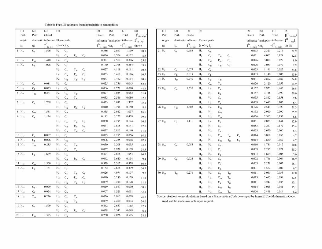
(1) (2) (3) (4) (5) (6) (7) (8) (1) (2) (3) (4) (5) (6) (7) (8)

Path Path Global Direct Path Total [IT

(i-->j)p/ Path Path Global Direct Path Total [IT

(i-->j)p/

origin destinationinfluence Elementarypaths influence *multiplier =influence IG

(i-->j)] origin destinationinfluence Elementarypaths influence *multiplier =influence IG

(i-->j)]

(i) (j) IG

(i-->j) ID

(i-->j)p *Mp =IT

(i-->j)p(in %) (i) (j) I

G(i-->j) I

D(i-->j)p *Mp =I

T(i-->j)p

(in %)

1 H0 Ca 1,596 H0 Ca 0,386 2,897 1,119 70,1 21 H6 Cs 0,988 H6 Cs 0,093 2,321 0,216 21,9

H0 Cm Pm Ca 0,036 3,704 0,132 8,3 H6 Ca Tm Cs 0,031 4,002 0,124 12,5

2 H0 Cm 1,448 H0 Cm 0,321 2,512 0,806 55,6 H6 Cm Pm Cs 0,026 3,051 0,079 8,0

3 H0 Cs 1,078 H0 Cs 0,130 2,798 0,364 33,8 H6 Cm Tm Cs 0,026 3,051 0,079 7,9

H0 Ca Tm Cs 0,027 4,118 0,111 10,3 22 H6 Ce 0,077 H6 Ce 0,023 1,191 0,027 34,8

H0 Cm Pm Cs 0,033 3,462 0,116 10,7 23 H6 Ch 0,019 H6 Ch 0,003 1,140 0,003 15,9

H0 Cm Tm Cs 0,033 3,462 0,114 10,6 24 H6 Tm 0,249 H6 Ca Tm 0,031 2,802 0,087 34,8

4 H0 Ce 0,081 H0 Ce 0,025 1,756 0,043 52,8 H6 Cm Tm 0,026 2,120 0,055 21,9

5 H0 Ch 0,023 H0 Ch 0,006 1,721 0,010 44,9 25 Htr Ca 1,655 Htr H0 Ca 0,152 2,923 0,443 26,8

6 H0 Tm 0,261 H0 Ca Tm 0,027 3,035 0,082 31,4 Htr H13 Ca 0,157 3,126 0,490 29,6

H0 Cm Tm 0,033 2,586 0,086 32,7 Htr H45 Ca 0,055 2,862 0,158 9,6

7 H13 Ca 1,738 H13 Ca 0,423 3,092 1,307 75,2 Htr H6 Ca 0,039 2,682 0,105 6,4

H13 Cm Pm Ca 0,040 3,798 0,150 8,6 26 Htr Cm 1,503 Htr H0 Cm 0,126 2,541 0,320 21,3

8 H13 Cm 1,581 H13 Cm 0,355 2,922 1,037 65,6 Htr H13 Cm 0,132 2,960 0,390 25,9

9 H13 Cs 1,174 H13 Cs 0,142 3,227 0,458 39,0 Htr H45 Cm 0,056 2,365 0,133 8,8

H13 Ca Tm Cs 0,030 4,195 0,124 10,6 27 Htr Cs 1,116 Htr H0 Cs 0,051 2,829 0,144 12,9

H13 Cm Pm Cs 0,037 3,815 0,141 12,0 Htr H13 Cs 0,053 3,267 0,172 15,4

H13 Cm Tm Cs 0,037 3,815 0,140 11,9 Htr H45 Cs 0,023 2,670 0,060 5,4

10 H13 Ce 0,087 H13 Ce 0,025 2,255 0,056 64,1 Htr H13 Cm Pm Cs 0,014 3,860 0,053 4,7

11 H13 Ch 0,026 H13 Ch 0,008 2,225 0,018 67,8 Htr H13 Cm Tm Cs 0,014 3,860 0,052 4,7

12 H13 Tm 0,285 H13 Ca Tm 0,030 3,208 0,095 33,3 28 Htr Ce 0,083 Htr H0 Ce 0,010 1,781 0,017 20,8

H13 Cm Tm 0,037 2,978 0,109 38,3 Htr H13 Ce 0,009 2,287 0,021 25,3

13 H45 Ca 1,639 H45 Ca 0,374 2,818 1,054 64,3 Htr H45 Ce 0,003 1,609 0,005 5,6

H45 Cm Pm Ca 0,042 3,640 0,154 9,4 29 Htr Ch 0,024 Htr H0 Ch 0,002 1,746 0,004 16,9

14 H45 Cm 1,560 H45 Cm 0,379 2,317 0,878 56,3 Htr H13 Ch 0,003 2,258 0,007 28,1

15 H45 Cs 1,151 H45 Cs 0,152 2,618 0,399 34,7 Htr H45 Ch 0,001 1,562 0,002 6,7

H45 Ca Tm Cs 0,026 4,074 0,107 9,3 30 Htr Tm 0,271 Htr H0 Ca Tm 0,011 3,061 0,033 12,0

H45 Cm Pm Cs 0,040 3,280 0,129 11,2 Htr H0 Cm Tm 0,013 2,615 0,034 12,5

H45 Cm Tm Cs 0,039 3,280 0,128 11,1 Htr H13 Ca Tm 0,011 3,242 0,036 13,1

16 H45 Ce 0,079 H45 Ce 0,019 1,567 0,030 38,6 Htr H13 Cm Tm 0,014 3,015 0,041 15,1

17 H45 Ch 0,024 H45 Ch 0,007 1,521 0,011 43,1 Htr H45 Cm Tm 0,006 2,448 0,014 5,2

18 H45 Tm 0,276 H45 Ca Tm 0,026 2,963 0,078 28,1 Source: Author's own calculations based on a Mathematica Code developed by himself. The Mathematica Code

H45 Cm Tm 0,039 2,400 0,094 34,0 used will be made available upon request.

19 H6 Ca 1,599 H6 Ca 0,442 2,637 1,165 72,9

H6 Cm Pm Ca 0,028 3,545 0,098 6,2

20 H6 Cm 1,325 H6 Cm 0,250 2,026 0,505 38,1

(i --> j )p

Table 6: Type III pathways from households to commodities

(i --> j )p

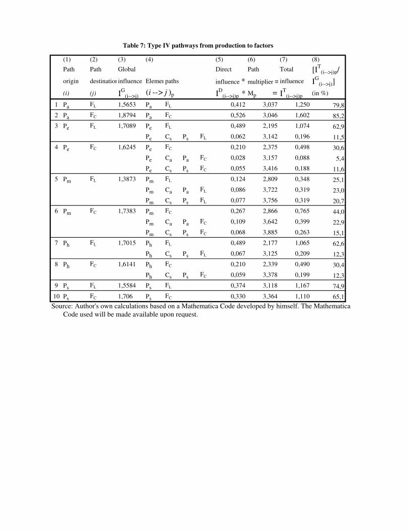
(1) (2) (3) (4) (5) (6) (7) (8)

Path Path Global Direct Path Total [IT

(i-->j)p/

origin destinationinfluence Elementarypaths influence * multiplier =influence IG

(i-->j)]

(i) (j) IG

(i-->j) ID

(i-->j)p * Mp = IT

(i-->j)p(in %)

1 Pa FL 1,5653 Pa FL 0,412 3,037 1,250 79,8

2 Pa FC 1,8794 Pa FC 0,526 3,046 1,602 85,2

3 Pe FL 1,7089 Pe FL 0,489 2,195 1,074 62,9

Pe Cs Ps FL 0,062 3,142 0,196 11,5

4 Pe FC 1,6245 Pe FC 0,210 2,375 0,498 30,6

Pe Ca Pa FC 0,028 3,157 0,088 5,4

Pe Cs Ps FC 0,055 3,416 0,188 11,6

5 Pm FL 1,3873 Pm FL 0,124 2,809 0,348 25,1

Pm Ca Pa FL 0,086 3,722 0,319 23,0

Pm Cs Ps FL 0,077 3,756 0,319 20,7

6 Pm FC 1,7383 Pm FC 0,267 2,866 0,765 44,0

Pm Ca Pa FC 0,109 3,642 0,399 22,9

Pm Cs Ps FC 0,068 3,885 0,263 15,1

7 Ph FL 1,7015 Ph FL 0,489 2,177 1,065 62,6

Ph Cs Ps FL 0,067 3,125 0,209 12,3

8 Ph FC 1,6141 Ph FC 0,210 2,339 0,490 30,4

Ph Cs Ps FC 0,059 3,378 0,199 12,3

9 Ps FL 1,5584 Ps FL 0,374 3,118 1,167 74,9

10 Ps FC 1,706 Ps FC 0,330 3,364 1,110 65,1

Source: Author's own calculations based on a Mathematica Code developed by himself. The Mathematica

Code used will be made available upon request.

(i --> j )p

Table 7: Type IV pathways from production to factors

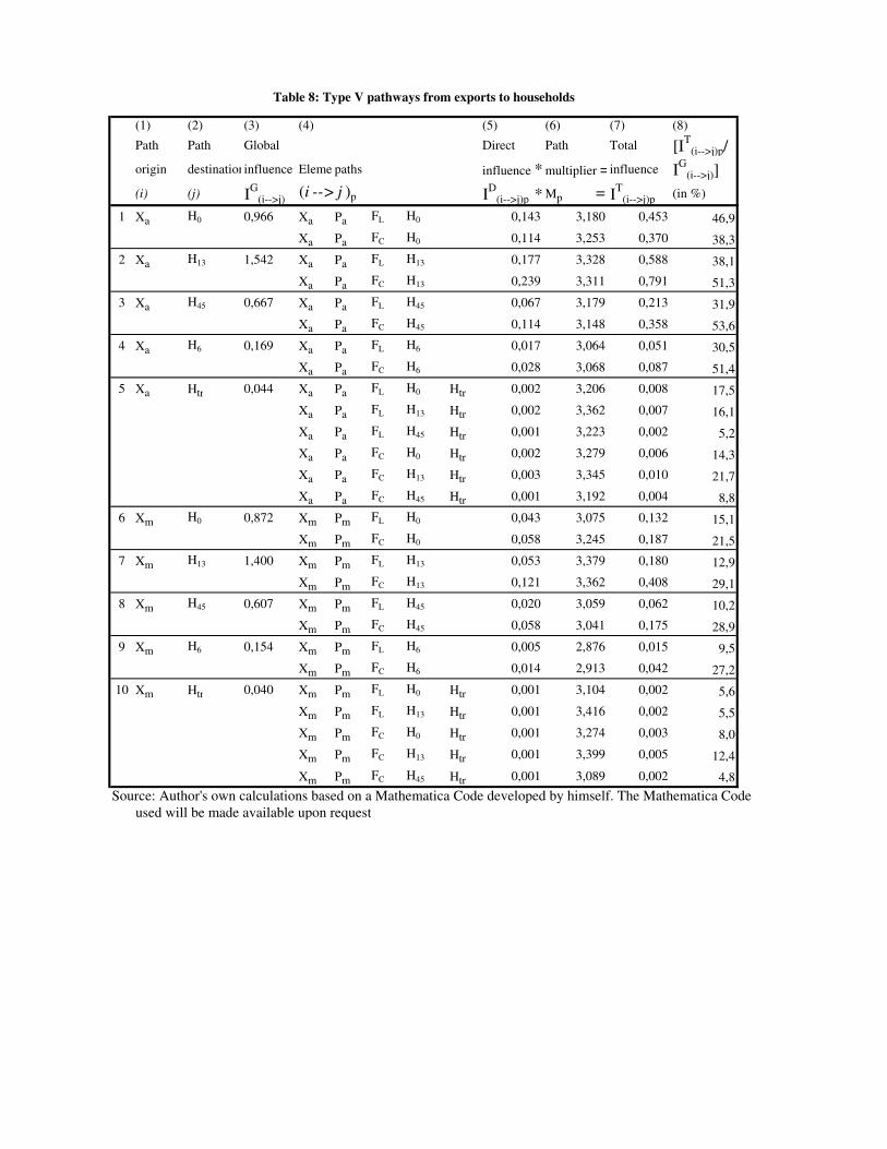
(1) (2) (3) (4) (5) (6) (7) (8)

Path Path Global Direct Path Total [IT

(i-->j)p/

origin destinationinfluence Elementarypaths influence * multiplier =influence IG

(i-->j)]

(i) (j) IG

(i-->j) ID

(i-->j)p * Mp = IT

(i-->j)p(in %)

1 Xa H0 0,966 Xa Pa FL H0 0,143 3,180 0,453 46,9

Xa Pa FC H0 0,114 3,253 0,370 38,3

2 Xa H13 1,542 Xa Pa FL H13 0,177 3,328 0,588 38,1

Xa Pa FC H13 0,239 3,311 0,791 51,3

3 Xa H45 0,667 Xa Pa FL H45 0,067 3,179 0,213 31,9

Xa Pa FC H45 0,114 3,148 0,358 53,6

4 Xa H6 0,169 Xa Pa FL H6 0,017 3,064 0,051 30,5

Xa Pa FC H6 0,028 3,068 0,087 51,4

5 Xa Htr 0,044 Xa Pa FL H0 Htr 0,002 3,206 0,008 17,5

Xa Pa FL H13 Htr 0,002 3,362 0,007 16,1

Xa Pa FL H45 Htr 0,001 3,223 0,002 5,2

Xa Pa FC H0 Htr 0,002 3,279 0,006 14,3

Xa Pa FC H13 Htr 0,003 3,345 0,010 21,7

Xa Pa FC H45 Htr 0,001 3,192 0,004 8,8

6 Xm H0 0,872 Xm Pm FL H0 0,043 3,075 0,132 15,1

Xm Pm FC H0 0,058 3,245 0,187 21,5

7 Xm H13 1,400 Xm Pm FL H13 0,053 3,379 0,180 12,9

Xm Pm FC H13 0,121 3,362 0,408 29,1

8 Xm H45 0,607 Xm Pm FL H45 0,020 3,059 0,062 10,2

Xm Pm FC H45 0,058 3,041 0,175 28,9

9 Xm H6 0,154 Xm Pm FL H6 0,005 2,876 0,015 9,5

Xm Pm FC H6 0,014 2,913 0,042 27,2

10 Xm Htr 0,040 Xm Pm FL H0 Htr 0,001 3,104 0,002 5,6

Xm Pm FL H13 Htr 0,001 3,416 0,002 5,5

Xm Pm FC H0 Htr 0,001 3,274 0,003 8,0

Xm Pm FC H13 Htr 0,001 3,399 0,005 12,4

Xm Pm FC H45 Htr 0,001 3,089 0,002 4,8

Source: Author's own calculations based on a Mathematica Code developed by himself. The Mathematica Code

used will be made available upon request

(i --> j )p

Table 8: Type V pathways from exports to households

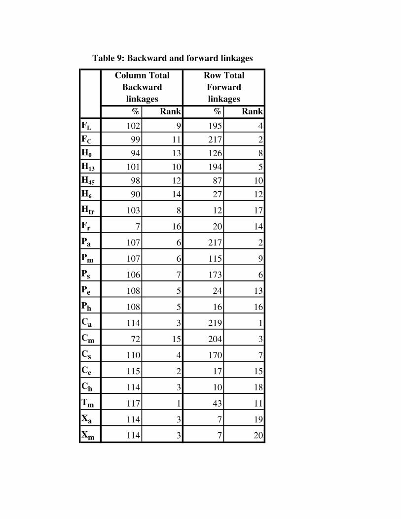
% Rank % Rank

FL 102 9 195 4

FC 99 11 217 2

H0 94 13 126 8

H13 101 10 194 5

H45 98 12 87 10

H6 90 14 27 12

Htr 103 8 12 17

Fr 7 16 20 14

Pa 107 6 217 2

Pm 107 6 115 9

Ps 106 7 173 6

Pe 108 5 24 13

Ph 108 5 16 16

Ca 114 3 219 1

Cm 72 15 204 3

Cs 110 4 170 7

Ce 115 2 17 15

Ch 114 3 10 18

Tm 117 1 43 11

Xa 114 3 7 19

Xm 114 3 7 20

Table 9: Backward and forward linkages

Row Total

Forward

linkages

Column Total

Backward

linkages