kriging interpolation in seismic attribute space applied to the … · kriging interpolation in...

General rights Copyright and moral rights for the publications made accessible in the public portal are retained by the authors and/or other copyright owners and it is a condition of accessing publications that users recognise and abide by the legal requirements associated with these rights.

Users may download and print one copy of any publication from the public portal for the purpose of private study or research.

You may not further distribute the material or use it for any profit-making activity or commercial gain

You may freely distribute the URL identifying the publication in the public portal If you believe that this document breaches copyright please contact us providing details, and we will remove access to the work immediately and investigate your claim.

Downloaded from orbit.dtu.dk on: Mar 22, 2020

Kriging interpolation in seismic attribute space applied to the South Arne Field, NorthSea

Hansen, Thomas Mejer; Mosegaard, Klaus; Schiøtt, Christian

Published in:Geophysics

Link to article, DOI:10.1190/1.3494280

Publication date:2010

Document VersionPublisher's PDF, also known as Version of record

Link back to DTU Orbit

Citation (APA):Hansen, T. M., Mosegaard, K., & Schiøtt, C. (2010). Kriging interpolation in seismic attribute space applied tothe South Arne Field, North Sea. Geophysics, 75(6), 31-41. https://doi.org/10.1190/1.3494280

https://doi.org/10.1190/1.3494280

https://orbit.dtu.dk/en/publications/080af409-366d-4a57-9555-89493292df99

https://doi.org/10.1190/1.3494280

KF

T

atsnni

itdmit

3

E

©

GEOPHYSICS, VOL. 75, NO. 6 �NOVEMBER-DECEMBER 2010�; P. P31–P41, 14 FIGS., 2 TABLES.10.1190/1.3494280

riging interpolation in seismic attribute space applied to the South Arneield, North Sea

. M. Hansen1, K. Mosegaard2, and C. R. Schiøtt3

vsaksXuavdvvac

ABSTRACT

Seismic attributes can be used to guide interpolation in-be-tween and extrapolation away from well log locations using forexample linear regression, neural networks, and kriging. Krig-ing-based estimation methods �and most other types of interpola-tion/extrapolation techniques� are intimately linked to distancesin physical space: If two observations are located close to one an-other, the implicit assumption is that they are highly correlated.This may, however, not be a correct assumption as the two loca-tions can be situated in very different geological settings. An al-ternative approach to the traditional kriging implementation issuggested that frees the interpolation from the restriction of thephysical space. The method is a fundamentally different applica-tion of the original kriging formulation where a model of spatial

D

cllcg

mcktsc

f

eived 21U Inforsen@gmsity of D

P31

Downloaded 20 Oct 2010 to 192.38.67.112. Redistribution subject to S

ariability is replaced by a model of variability in an attributepace. To the extent that subsurface geology can be described byset of seismic attributes, we present an automated multivariateriging-based interpolation method that is guided by geologicalimilarity rather than by the conventional distance measure inYZ space. Through a case study, kriging in attribute space issed to estimate 2D porosity maps from a number of well logsnd seismic attributes in the Danish North Sea. Cokriging pro-ides uncertainty estimates that are dependent on the primaryata locations in space, whereas kriging in attribute space pro-ides uncertainty estimates that reflect subsurface geologicalariability. The North Sea case study demonstrates that kriging inttribute space performs better than linear regression andokriging.

INTRODUCTION

Geophysical prospecting data zobs are often measured at a discretend limited set of locations u in space. Interpolation of such data ishen often used to provide an area-covering map, which indicates thepatial distribution of the parameter. Several interpolation tech-iques exist to provide such interpolation. Examples of such tech-iques, to name a few, are linear regression, inverse distance, splinenterpolation, and kriging-based interpolation.

An obvious way to increase the quality of an interpolated map is toncrease the density of direct data observations zobs. Often, however,he cost of measuring zobs is high and therefore prohibitive �e.g.,rilling of new exploration wells�. An alternative approach is toake use of cheaper information — for instance seismic data — that

n some way is linked or sensitive to changes in the primary parame-er of interest. Here, we will refer to such data as “attributes.”

Manuscript received by the Editor 28August 2009; revised manuscript rec1Formerly at Niels Bohr Institute, Copenhagen, Denmark; presently at DT

21, 2800 Lyngby, Denmark. E-mail: [email protected], thomas.mejer.han2Technical University of Denmark, DTU Informatics, Technical Univer

-mail: [email protected], Copenhagen, Denmark. E-mail: [email protected] Society of Exploration Geophysicists.All rights reserved.

istance in physical space as a guide for interpolation

Most interpolation techniques use a measure of distance in physi-al space as a measure of similarity and hence as a guide for interpo-ation. The implicit assumption is that an observed parameter at twoocations separated by a small distance have similar values. In someases, this may be a valid criterion for interpolation. However, in aeological scenario, this approach has some significant drawbacks.

Consider two locations, A and B, and primary data, zA and zB,easured at A and B, respectively. Assume that A and B are located

lose to each other in physical space. If no other information isnown about A and B, one could expect zA to be strongly correlatedo zB. However, A and B may be located in very different geologicalettings, if for example, A and B are separated by a fault. In such aase, one would not necessarily expect zA to be correlated to zB.

On the other hand, assume that the locations A and B are locatedar away from each other in physical space. Intuitively one would

April 2010; published online 20 October 2010.matics, Technical University of Denmark, Richard Petersens Plads, Bygning

ail.com.enmark, Richard Petersens Plads, Bygning 321, 2800 Lyngby, Denmark.

EG license or copyright; see Terms of Use at http://segdl.org/

pac

ilc

peefs

M

ea12spwpttgong

lataplera

udsairits

Acmc

lst

Ti

wzwtt

Fotb1

Z�teastecK

etmH

w

Kvkco

P32 Hansen et al.

erhaps not expect zA to be similar to zB, but ifAand B are situated inlmost identical geological settings, one could argue that zA and zB

ould indeed be strongly correlated.This simple example illustrates that rather than using the distance

n physical space, it may sometimes be desirable to perform interpo-ation based on geological similarity. It is this viewpoint that we willonsider in this paper.

We will assume that we have access to only a limited number ofrimary data �e.g., well data�, but that an exhaustive set of area-cov-ring attributes �e.g., seismic data/attributes� are available. To thextent that the attributes available are sensitive to changes in subsur-ace geology, we will consider interpolation based on geologicalimilarity, as opposed to the distance in physical space.

ultivariate interpolation

Existing methods for high-dimensional interpolation include lin-ar regression �Hampson et al., 2001; Russell et al., 2002; Hansen etl., 2008�, spline interpolation, nearest neighbor, cokriging �Doyen,988�, and neural networks �Hampson et al., 2001; Russell et al.,002; Pramanik et al., 2004; Herrara et al., 2006�. Some comparativetudies of these methods are available. Hampson et al. �2001� com-are the use of linear regression, multilayer feed-forward neural net-orks and probabilistic neural networks. Russell et al. �2002� com-are generalized regression neural networks and radial basis func-ion networks for prediction of log properties from seismic at-ributes. Pramanik et al. �2004� compare the application of linear re-ression, neural networks, cokriging with impedance, and cokrigingf actual porosity estimates with a porosity map obtained using aeural network. Herrara et al. �2006� uses a combination of linear re-ression and neural networks.

As opposed to most of the listed methods, kriging-based interpo-ation produces not only an estimate of the primary parameter, butlso an estimate of the local uncertainty. Cokriging has been appliedo porosity estimation, using an exhaustive map of acoustic imped-nce as secondary data �Doyen, 1988�. Cokriging provides an im-rovement compared to traditional kriging in that it allows modelingocal variability conditioned by secondary variables. Still, the infer-nce of the covariance model used to perform kriging is intimatelyelated to distance measures in physical space and implies a certainmount of smoothness to the kriging mean and variance results.

As an alternative to the methods described above, we propose totilize a variant of kriging that is free of constraints from physicalistance. We assign all primary data to a point in the high-dimen-ional space spanned by the considered attributes, assuming that thettributes �secondary data� are available everywhere in the area ofnvestigation. Note that the spatial X-, Y-, and Z components can beegarded as attributes and therefore can be included in the estimationf we wish. We then suggest performing univariate kriging interpola-ion directly in the attribute space, as opposed to the physical XYZpace.

We apply the method in a case study using data from the Southrne field in the North Sea. We demonstrate how a map of porosity

an be estimated from a number of well log measurements and seis-ic attributes extracted from a 3D seismic data set. This result is

ompared to cokriging using acoustic impedance as secondary data.


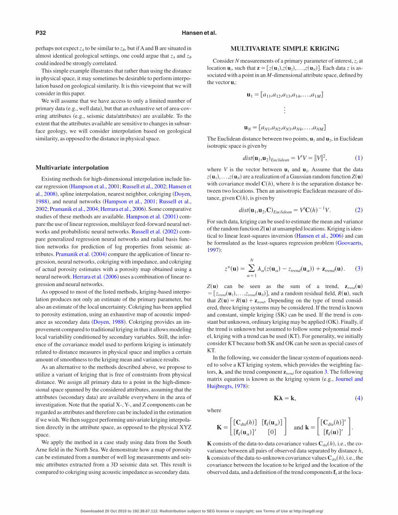
MULTIVARIATE SIMPLE KRIGING

Consider N measurements of a primary parameter of interest, zi atocation ui, such that z� �z�u1�,z�u2�, . . . ,z�uN��. Each data z is as-ociated with a point in an M-dimensional attribute space, defined byhe vector ui:

u1� �a11,a12,a13,a14, . . . ,a1M�

]

uN� �aN1,aN2,aN3,aN4, . . . ,aNM�

he Euclidean distance between two points, u1 and u2, in Euclideansotropic space is given by

dist�u1,u2�Euclidean�VtV� �V�2, �1�

here V is the vector between u1 and u2. Assume that the data�u1�, . . . ,z�uN� are a realization of a Gaussian random function Z�u�ith covariance model C�h�, where h is the separation distance be-

ween two locations. Then an anisotropic Euclidean measure of dis-ance, given C�h�, is given by

dist�u1,u2,C�Euclidean�VtC�h��1V . �2�

or such data, kriging can be used to estimate the mean and variancef the random function Z�u� at unsampled locations. Kriging is iden-ical to linear least-squares inversion �Hansen et al., 2006� and cane formulated as the least-squares regression problem �Goovaerts,997�:

z*�u�� 1

N

��z�u��ztrend�u��ztrend�u� . �3�

�u� can be seen as the sum of a trend, ztrend�u��ztrend�u1�, . . . ,ztrend�uN��, and a random residual field, R�u�, such

hat Z�u��R�u��ztrend. Depending on the type of trend consid-red, three kriging systems may be considered. If the trend is knownnd constant, simple kriging �SK� can be used. If the trend is con-tant but unknown, ordinary kriging may be applied �OK�. Finally, ifhe trend is unknown but assumed to follow some polynomial mod-l, kriging with a trend can be used �KT�. For generality, we initiallyonsider KT because both SK and OK can be seen as special cases ofT.In the following, we consider the linear system of equations need-

d to solve a KT kriging system, which provides the weighting fac-ors, �, and the trend component ztrend for equation 3. The followingatrix equation is known as the kriging system �e.g., Journel anduijbregts, 1978�:

K��k, �4�

here

K��Cdtd�h�� fk�u��fk�u�� 0� � and k��Cdtu�h��

�fk�u�� .

consists of the data-to-data covariance values Cdtd�h�, i.e., the co-ariance between all pairs of observed data separated by distance h,consists of the data-to-unknown covariance values Cdtu�h�, i.e., the

ovariance between the location to be kriged and the location of thebserved data, and a definition of the trend components f at the loca-
k

tapis

ao

wp�

kpft

kbaoeas

C

art

tFTe

rvtntcpia

D

a

Grtssmr

wsStadfi

gntvAttcoes

A

aoipeec

sDiInepanRicnoaust

Kriging interpolation in attribute space P33

ion to be kriged. If a constant trend is considered, then K�Cdtd�h�nd k�Cdtu�h� and the kriging system above is reduced to the sim-le kriging system for which we shall provide the solution below. �s the vector of kriging weights of equation 3, associated with the ob-erved data. Kriging weights are found using

��K�1k �5�

nd used to estimate the local Gaussian probability density of theutcome of the random function at the unsampled location:

�KT�zt�� 6�

� KT2 �C�0��kt�, �7�

here �� 1, . . . ,�N�, �� is the a priori mean value, �KT is mean ex-ected value, and � KT is the standard deviation. See e.g., Goovaerts1997� for details on the solution of kriging systems.

As can be seen from the above equations, in order to solve theriging system, one must choose a model for the trend fk and com-ute the covariance C�h� using some predefined covariance modelrom the computed separation distance h between pairs of data loca-ions.

One way of choosing the trend model fk�u� can be based on priornowledge of the system or on observations.Alternatively, fk�u� cane chosen as the outcome of another interpolation method, as for ex-mple, the trend model presented by Hansen et al. �2008�. The meth-d we present here will model the variability around this trend mod-l. In this paper, we focus on the inference of the covariance modelnd the application to kriging in the high-dimensional attributepace.

ovariance model, shape, and range

Cdtd�h� and Cdtu�h� contain covariance values as a function of sep-ration distance h. To compute these, one needs to select some cova-iance model to describe the spatial correlations in the residual �non-rend� part of the random function R�u�.

The choice of covariance model is very important because it de-ermines the part of the interpolation not accounted for by the trend.urthermore, it determines the estimated interpolation variance.herefore we pay special attention to the choice of covariance mod-l.

For lower-dimensional problems �up to three dimensions� a cova-iance model can be inferred directly from data, using classical semi-ariogram analysis �e.g., Goovaerts, 1997�. To provide objective es-imates for higher dimensional problems, we suggest defining a ge-eric choice of covariance model and selecting an optimization cri-erion that can be used to infer the parameters of this model. Thehoice of optimization criterion should result in both reliable inter-olation and uncertainty estimates. In the following, we will discussn detail how to choose such a generic covariance model and suggestn approach to infer the parameters of this model.

efining a generic covariance model for multivariate data

The most widely considered analytical covariance model typesre the Nugget, Gaussian, Exponential, and Spherical models �e.g.,


oovaerts, 1997�. They differ mostly in the behavior at small sepa-ation distances, except for the Nugget model, which implies no spa-ial correlation, but only small scale variability below the smallesteparation distance. The Gaussian model tends to provide the mostmooth interpolation result. A generic definition of a covarianceodel, given any of these covariance types V with a sill S and a rangeis given by

C�h��SV�r��h�, �8�

here h is the separations distance between two locations. We con-ider the combination of a Nugget model with one of the Gaussian,pherical, or Exponential covariance models. We will assume that

he global sill value S �i.e., the sum of the sills of the selected covari-nce models� is known and is equal to the variance of the detrendedata observations such that a generic covariance model can be de-ned:

C�� ,S,r,M,h�� SNug�0�� 1�� SV�r��h� . �9�

The nugget fraction � is a convenient measure to use. If the nug-et fraction is 1, the combined covariance model is identical to a pureugget model �i.e., a covariance model suggesting no spatial correla-ion�. In this case, only the trend model is estimated, and the krigingariance will be constant and equal to the size of the global sill value.nugget fraction of 0 suggests that there is no small-scale variabili-

y. In this way, the nugget fraction controls the relative weight of therend and the spatial correlation in the kriging estimation. The spatialorrelation is controlled by the range of the non-Nugget componentf the covariance model. A covariance model with zero range isquivalent to a pure nugget model. An infinitely long range will re-ult in an interpolation result equal to linear interpolation.

nisotropy

The isotropic formulation of the covariance model in equation 9 isdequate to specify the covariance model for the kriging system withnly 1 attribute �i.e., in R1�. For higher dimensions, however, an an-sotropic covariance model is usually needed. In the context of theresent work, there is little chance that an isotropic covariance mod-l would properly describe data in an attribute space spanned by, forxample, seismic impedance and two-way travel time, simply be-ause these two attributes are measured on different scales.

Anisotropic covariance models are well described in the geo-tatistical literature for up to three dimensions �e.g., Chiles andelfiner, 1999�.Anisotropy can be defined by a combination of scal-

ng for each dimension and a rotation of the coordinate system axes.n the simplest case, the anisotropy axes coincide with the coordi-ate axes, and hence only scaling is applied and rotation is not need-d �Chiles and Delfiner, 1999�. We will refer to this form of anisotro-y as “scaling anisotropy.” Only the range along each coordinatexis needs to be specified. In this case only, the range along each axiseeds to be specified. Thus M range values need to be selected in

M. The more general “elliptic” anisotropy, making use of both scal-ng and rotation, will be applied if the anisotropy axes do not coin-ide with the coordinate axes. In this case, the rotation of the coordi-ate system is performed using a transformation matrix. The numberf angles needed to completely define the rotation is 0 in R1, 1 in R2,nd 3 in R3. Hence, �M � �M �1�� /2 angles are needed in RM. It isnfeasible to infer meaningful values to all angles in higher dimen-ions, so we will only consider scaling anisotropy in the remainder ofhis paper.


so

Ict�m�ob

I

mabaom

ns�h1cú

oi�sw

wpssúwa

tnmtm

NiauepppFs

dlT

a

Fsta

P34 Hansen et al.

Assume that the range parameters are r� �r1,r2, . . . ,rM� in RM, theill is S, and the nugget fraction of the sill is � . The general form ofur covariance model will then be

C�� ,S,r�� SNug�0�� 1�� SV�r��h� . �10�

n RM this corresponds to M �2 parameters to be inferred. If the ofovariance model type is known, the number of unknown parame-ers is M �1. Figure 1a shows an example of a 1D covariance model� �0.3, S�1, r�1� and Figure 1b an example of a 2D covarianceodel with scaling anisotropy as defined above �� 0.3, S�1, r�1,2��. Note that the relation between the semivariogram �most

ften used in geostatistics�, � �h�, and the covariance model is giveny � �h��C�0��C�h� �see Figure 1a�.

nference of a multivariate covariance model

In a classical geostatistical work flow an experimental covarianceodel is calculated from observations. Then an analytical covari-

nce model is fitted to the experimental covariance model. This cane done either manually or using an automated approach for covari-nce fitting, as suggested by for example, Cressie �1985�. This meth-d, however, relies on subjective choices and requires relativelyany data to compute a reliable experimental covariance model.Pardo-Igúzquiza �1998� compares a number of different tech-

iques for inferring the range of a covariance models. He demon-trates that the cross-validation-based maximum likelihood methodSamper and Neuman, 1989a, b, c�, and the regular maximum likeli-ood approach �ML� �Kitanidis and Lane, 1985; Pardo-Igúzquiza,997; Diggle et al., 2003� provide almost equally good results. Foromputational efficiency, we consider the ML method of Pardo-Ig-zquiza �1997, 1998�.

Assume that the subsurface can be seen as a realization of a 2ndrder stationary Gaussian random field and that a sample of the real-zation is available in form of N direct observations of z

�z1,z2, . . . ,zN�. Then the negative log-likelihood Lnllf that these ob-ervations can be seen as a realization of a Gaussian random fieldith covariance CM is given as

1 0.5 0Distance (attrib

1.0

0.8

0.6

0.4

0.2

0.0

0.2

0.4

0.6

0.8

1.0

Dis

tanc

e(a

ttrib

ute

2)

0 0.2 0.4 0.6 0.8Distance (m)

1 1.2

1.0

0.8

0.6

0.4

0.2

0.0

Cov

aria

nce

Sem

ivar

ianc

e

1

0.8

0.6

0.4

0.2

0

) b)

igure 1. �a� 1D �’0.3 Nug� � .7 Sph�1�’� covariance �thick soponding semivariogram �thin gray line�. The nugget is indicated byhe range by the dashed line. �b� 2D �’0.3 Nug�0.7 Sph�1,0.5�’� exnce model defined by equation 10.


Lnllf�Q,z,ztrend��N

2�ln�2��1� ln�N��

1

2lnQ

�N

2ln��z�ztrend�TQ�1�z�ztrend��,

�11�

here Q�CM /CM�0� and ztrend is the trend model at the observationoints. In the maximum likelihood approach, the parameters of theubsurface covariance model can be found by minimizing expres-ion 11 with respect to the components of Q, z, and ztrend �Pardo-Ig-zquiza, 1997, 1998�. For the purpose of kriging in attribute space,e minimize equation 11 to infer the nugget fraction, ranges for each

ttribute direction and the covariance model type of equation 10.We thus suggest to perform univariate kriging in a multivariate at-

ribute space �equations 4–7�, based on automatic inference of a ge-eric covariance model �equation 10� using maximum likelihoodaximization of equation 11. In the following, we apply the method

o estimate a 2D map of porosity using attributes obtained from seis-ic data.

CASE STUDY AND DISCUSSION

The South Arne Field is a chalk reservoir situated in the Danishorth Sea �Mackertich and Goulding, 1999�. The oil-bearing chalk

s characterized by porosities in the range 20-45 porosity units �PU�s interpreted from well log data. Estimates of porosity are key val-es in the assessment of in-place oil volumes. This case study utiliz-s kriging in multiattribute space as a tool for estimating reservoirorosity guided by seismic attributes. For simplicity, we considerorosity variation in 2D. However, the methodology is readily ex-andable to 3D. In this study, we focus on the main reservoir, the Torormation, which is of Maastrichtian age and is located in the chalkection of the SouthArne Field in the North Sea.

In total, we have access to nine attributes extracted from seismicata in a dense, geographical 2D XY-grid consisting of 37,791 dataocations. The two-way travel time �TWT�, “depths” to top �Topor�, and base �Base Tor� have been established directly from the

seismic data. Based on these data, the thickness ofthe Tor formation is computed and used as an at-tribute. At Top Tor, the amplitude �Top Tor Am-plitude� and the dip �Top Tor Dip� have been ex-tracted as attributes. The acoustic impedance at-tribute �AI�, derived from the seismic waveforms,is available everywhere. Thus, five seismicallyrelated attributes are available �Top Tor, Base Tor,Top TorAmplitude, Top Tor Dip,AI�. In addition,we consider the three �spatial� coordinated UTMX, UTM Y, and UTM Z as attributes. Figure 2a-ishows each attribute �and thereby the areal cover-age of the study area�, and Figure 2j shows the lo-cation and value of porosity measurements. Notethat for all 2D plots, we have rotated the originalUTM X-UTM Y axes to fit the layout of the data.The original direction to the North is indicated by

1

1

0.9

0.8

0.7

0.6

0.5

0.4

0.3

0.2

0.1

0

Cov

aria

nce

� and corre-tted line and

of the covari-

ute 1)0.5

lid linethe do

ample


tmoapa

D

wbt3g3bemtaata3wpttl

A

sh

1

pTftddo

2

tsmcswtwv

mrgtHeut

Ft

nes for

Cov

aria

nce


he arrow on Figure 2j. We consider the well-site porosity measure-ents as sparsely sampled values of a porosity function, defined

ver the �up to� nine-dimensional attribute space. We use kriging inttribute space as outlined above to estimate the porosity in form of arobability distribution at every unsampled location in the studyrea.

istance in attribute space as a measure of similarity

Figure 3 shows the distance from one location �white� to every-here else in the study area, calculated in the attribute space definedy X andY �Figure 3a� andAI �Figure 3c�, respec-ively. The distance in AI attribute space �Figurec� describes better the variation in subsurfaceeology than the spatial distance measure �Figurea�. Standard kriging-based interpolation isased on distance-dependent covariances. As anxample, we consider an exponential covarianceodel with a range of 20% of the maximum dis-

ance in each considered attribute space �3200 mnd 7.5105 kg /m2 s, respectively�. Figure 3bnd d shows the corresponding covariance func-ion centered at one location, everywhere in therea. With respect to theAI attribute space, Figured clearly shows that locations correlated to thehite circle follow a complex geological �andlausible� pattern, in contrast to the physical-dis-ance-based covariance �Figure 3b�. Thus, at-ribute-guided kriging interpolation tends to fol-ow geological similarity.

utomatic inference and interpolation

The methodology of using kriging in attributepace is similar whether a one-dimensional or aigher-dimensional attribute space is considered:

Normal score transformation

Kriging assumes that data can be seen as sam-les from a continuous Gaussian distribution.herefore we make use of a normal score trans-

ormation of the porosity data, which transformhe porosity data to a set of Gaussian distributedata with mean 0 and variance 1. The transformedata are referred to as the normal scores of theriginal porosity data.

Choice of trend model

Using kriging involves choosing or modeling arend model as discussed previously. The krigingystem is then applied to the residuals of the nor-al score, with the trend removed. Because the

ovariance model specified for the KT-krigingystem describes the covariance of the residuals,e must solve the kriging system in order to find

he residuals related to a given trend model. Thuse need to know the trend model to infer the co-ariance model for the residuals. Further, the esti-

Y(k

m)

18

16

14

12

10

8

6

4

2

04

X (km)20

Y(k

m)

18

16

14

12

10

8

6

4

2

04

X (km)20

a)

f)

Figure 2. �a–ivalues and blulines are iso li

Y(k

m)

18

16

14

12

10

8

6

4

2

0420

X (km)

a)

Figure 3. Distthe white circmodel and in �


ate of uncertainty obtained by the kriging system relates only to theesiduals, and is not affected by the trend model. Therefore we sug-est to avoid calculation of the trend model as part of the kriging sys-em and instead use and alternative method �e.g., Russell et al., 1997;ampson et al., 2001; Russell et al., 2002; Hansen et al., 2008; Ped-

rsen-Tatalovic et al., 2008�. Given such a trend model, we suggestsing the presented method to improve the trend model by modelinghe variations away from the trend.

For this case study, we will consider a very simple trend model.or all directions, except for the AI attribute, we choose a constant

rend model, and for theAI attribute, we choose a linear trend model.

4X (km)

20

Y(k

m)

18

16

14

12

10

8

6

4

2

04

X (km)20

Y(k

m)

18

16

14

12

10

8

6

4

2

04

X (km)20

Y(k

m)

18

16

14

12

10

8

6

4

2

04

X (km)20

4X (km)

20

Y(k

m)

18

16

14

12

10

8

6

4

2

04

X (km)20

Y(k

m)

18

16

14

12

10

8

6

4

2

04

X (km)20

Por

osity

units

40

35

30

25

20

15

10

5

N

Y(k

m)

18

16

14

12

10

8

6

4

2

04

X (km)20

c) d) e)

h) i) j)

ble attributes within the test area. Red colors indicate relative highrs relative low values. �j� Observed porosity from well logs. SolidUTM X�5.785e�6 m and UTM Y�6.214e�6 m.

1

0.9

0.8

0.7

0.60.5

0.40.3

0.2

0.1

Y(k

m)

18

16

14

12

10

8

6

4

2

0420

X (km)

Cov

aria

nce

x 106

54.543.532.521.510.50

Y(k

m)

18

16

14

12

10

8

6

4

2

0420

X (km)

Dis

tanc

e(a

cous

ticim

peda

nce) 1

0.9

0.8

0.7

0.6

0.5

0.4

0.3

0.2

0.1

Y(k

m)

18

16

14

12

10

8

6

4

2

0420

X (km)

b) c) d)

�a� X-Y space and �c� AI attribute space to the location denoted byariance computed in X-Y space using an �b� isotropic covariance

pace.

Y(k

m)

18

16

14

12

10

8

6

4

2

0

Y(k

m)

18

16

14

12

10

8

6

4

2

0

b)

g)

� Availae colo

Dis

tanc

e(k

m)

16

14

12

10

8

6

4

2

0

ance inle. Covd�AI s


TrC

3

trFtep

4

el

5

bbnts

bpntsme

K

ssUs“ddw�tddnis

udbadftf

T

D

1

2

3

4

5

6

f

Fml

P36 Hansen et al.

he latter choice is based on the well-known fact that a strong linearelation exists between acoustic impedance and porosity in thehalk section of the North Sea.

Inference of the covariance model in attribute space

The actual optimization of expression 11 is done using a combina-ion of global and local optimization. A Metropolis-Hastings algo-ithm is initially used to sample Lnllf of equation 11, such as shown inigure 4. Note that a well-defined maximum can be located. Using

he set of covariance model parameters with the location of the high-st Lnllf as a starting point, a local search is then performed to find theoint of maximum likelihood.

Kriging in normal score attribute space

Kriging in normal-score attribute space is a matter of solvingquations 4–7 to obtain an estimate of the normal scores at unknownocations in attribute space.

able 1. Mean prediction error of blind data considering the

ata set MM1 CoKrig A

�d�2� 3.6 3.6

�d�5� 2.7 2.7

�d�10� 3.6 3.6

�X�5.785e�5 m� 3.5 3.5

�Y�6.214e�6 m� 8.7 8.7

�Y�6.212e�6 m� 5.1 5.0

Columns 2 and 3 refer to the use of colocated �MM1� and full �CoKers to the use of a linear trend model �AI trend�. The last four column

0 2 4 6 8 10Range (AI units) 6

x 10

1.0

0.9

0.8

0.7

0.6

0.5

0.4

0.3

Nug

getf

ract

ion

igure 4. Maximum likelihood �ML� distribution of the covarianceodel parameters in AI attribute space. Darker colors reflects high

ikelihood and lighter colors low likelihood.


Inverse normal score transformation

An actual porosity estimate in original porosity units is obtainedy back-transforming the kriging estimates. The result of kriging-ased interpolation can now be obtained by visualizing the inverseormal score transform in the 2D UTM X-UTM Y coordinate sys-em. Thus, the kriging is performed in attribute space, but data are vi-ualized in spatial �2D� space.

The kriging result is not just the interpolated values of porosity,ut a local probability distribution providing the local distribution oforosity, conditioned to all observations. Because we make use of aormal score transformation of data, the shape of the local probabili-y distribution of porosity is usually not Gaussian. We shall laterhow examples of how to estimate both confidence intervals andaps showing the probability that the porosity is within certain rang-

s.

riging in high-dimensional attribute space

To investigate the performance of the proposed method, we con-ider five attribute sets in which we perform kriging in attributepace: �AI�, �UTM X, UTM Y�, �UTM X, UTM Y, AI�, �All butTM X and UTM Y�, and �all attributes�. We also consider six sub-

ets of the original 213 available porosity measurements as observedknown” porosity data: 1� every 2nd, 2� every 5th, and 3� every 10thata point; 4� all data points with UTM X 5.785e�5 m; 5� allata points with UTM Y 6.214e�6 m; and 6� all data pointsith UTM Y �6.214e�6 m. See Figure 2j for iso lines for UTM X5.785e�5 m and UTM Y �6.214e�6 m. Each data subset

hen considers �106, 53, 21, 178, 99, 114� observations as knownata. The rest of the available porosity data are referred to as “blind”ata and shall be used for comparison. Kriging in attribute space isow performed for all combinations of data and attribute subsets, bynferring the covariance model in attribute space for each data sub-et, followed by kriging of the porosity at the blind data locations.

Table 1 reports the average prediction error of the blind data notsed in optimization for different choices of selected attributes andata subset. A significant result in Table 1 is that increasing the num-er of considered attributes generally leads to a decrease in the aver-ge prediction error of the data not used in the optimization. Intro-ucing an attribute with no apparent relation to the primary data, asor example, the amplitude attribute, does not reduce the quality ofhe final prediction result. The maximum likelihood approach for in-erring the covariance model therefore seems very robust with re-

ubsets and different attributes and methods.

X,Y X,Y,AI All but XY ALL

1.8 1.8 2.0 1.7

2.7 2.5 2.5 2.3

4.1 3.1 3.2 3.2

5.6 3.1 3.2 3.2

11.6 8.5 6.4 8.2

4.3 3.3 4.0 3.4

kriging in XY space, withAI as a secondary attribute. Column 4 re-to kriging in attribute space using the given attributes.

data s

I trend

3.5

3.4

3.5

4.4

6.7

3.6

rig� cos refer


sfertbiHcce

aspauai

eccssit

rktAiHidsat

U

smrlkbocfttaneutr

a

d

Fdsa


pect to noisy/unrelated attributes: If such attributes exist, the in-erred covariance model for that specific attribute direction will haveither a large nugget or a very short range, indicating little to no cor-elation for changes in the attribute and therefore little to no effect onhe final prediction. Reducing the number of considered attributesased on feature extraction �e.g., Hampson et al., 2001� may be a val-d approach if the number of available attributes becomes very large.owever, for the data set used in this study our findings above indi-

ate that feature extraction is not needed because the blind error de-reases as attributes �believed a priori to be less significant� are add-d to the list of attributes considered by the method.

The lowest prediction error of the blind data is at a level of 1.7 PUnd is found when considering all the available attributes for dataubset 1. This is a large improvement over the simple, traditional ap-roach of using a linear relationship between acoustic impedancend porosity, which results in a prediction error of about 3.5 PU. Fig-re 5 shows the estimated mean porosity using all attributes avail-ble for all data subsets. Figure 6 shows the estimated mean porosityn a smaller region for easier comparison.

Figure 7 shows the estimated mean porosity using all attributesxcept for the spatial attributes. From Table 1 it is seen that, whenonsidering all attributes but UTM X, UTM Y, and UTM Z, therossvalidation error is comparable to using all attributes and con-iderably lower than using simple linear regression. Thus, the pre-ented method provides relatively good results even when discard-ng the traditional spatial information that controls many interpola-ion algorithms.

It is clear from Figures 5–7 that theAI attribute plays an importantole in predicting the porosity, as should be expected due to thenown, strong correlation between acoustic impedance and porosi-y. Figure 8 shows the estimated mean porosity when not using theI attribute. For data subsets 1–4 the general trend of high porosity

n the northwest and lower porosity towards the southeast is found.owever, for the last two data subsets �5 and 6�, where data are split

nto a set of data toward the north and the south, respectively, krigingoes not perform very well �neither in physical space, nor in attributepace�. This is because there are no trends in the considered data toccount for the north-south observed variability in the porosity dis-ribution.

ncertainty estimates

The result of kriging in attribute space is notimply the mean estimate, but actually an esti-ate of the local probability distribution of po-

osity. Because the kriging is performed on a non-inear normal score transform of the data, theriging estimate of variance cannot be directlyack-transformed to an estimate of the variancef the porosity estimate. In fact, the estimated lo-al pdf of porosity is non-Gaussian in back-trans-ormed space. However, the kriging variance es-imate in normal score space is useful to visualizehe distribution of spatial uncertainty. As an ex-mple, Figure 9 shows the estimated variance inormal score space using all attributes for differ-nt subsets of data. Using data subset 1 �where thenknown data locations on average are closest tohe known data locations�, the uncertainty mapeflects the location of the known data locations

1 1.5

15.0

14.5

14.0

13.5

13.0

Y(k

m)

1 1.5

15.0

14.5

14.0

13.5

13.0

Y(k

m)

a)

d)

Figure 6. As Fsubsets 1–6 in


18

16

14

12

10

8

6

4

2

0

Y(k

m)

4X (km)20

18

16

14

12

10

8

6

4

2

0

Y(k

m)

4X (km)20

18

16

14

12

10

8

6

4

2

0

Y(k

m)

4X (km)20

18

16

14

12

10

8

6

4

2

0

Y(k

m)

4X (km)20

18

16

14

12

10

8

6

4

2

0

Y(k

m)

4X (km)20

18

16

14

12

10

8

6

4

2

0

Y(k

m)

4X (km)20

40

35

30

25

20

15

10

5

Por

osity

units

) b) c)

) e) f)

igure 5. Estimated porosity �mean� using all attributes for differentata subsets as hard data: �a� subset 1, �b� subset 2, �c� subset 3, �d�ubset 4, �e� subset 5, and �f� subset 6. Used and blind data locationsre indicated using white and black dots, respectively.

2 2.5 3X (km)

1 1.5 2 2.5 3X (km)

15.0

14.5

14.0

13.5

13.0

Y(k

m)

1 1.5 2 2.5 3

15.0

14.5

14.0

13.5

13.0

X (km)

Y(k

m)

2 2.5 3X (km)

1 1.5 2 2.5 3X (km)

15.0

14.5

14.0

13.5

13.0

Y(k

m)

1 1.5 2 2.5 3

15.0

14.5

14.0

13.5

13.0

X (km)

Y(k

m)

b) c)

e) f)

igure 5 �with same colorscale�, but zooming in on a smaller area. Hard data�a–f�.


iptcs

btltmbpPe

pl3

t

cmoNaqail

E

ttefl�l0lm

a

d

Fto

a

d

FAd

P38 Hansen et al.

n 2D �Figure 9a�. This is similar to the result when using kriging inhysical space, where the uncertainty map is related in a simple wayo the data locations. Because less data are available, Figure 9b and clearly shows that the uncertainty variance map tends to reflect theubsurface variation as given by the attributes available.

Actual uncertainties of porosity estimates can be obtained byack-transforming certain quantiles in the normal score space. Inhis way, probability maps of the porosity can be obtained. We be-ieve that, because the uncertainty estimates using kriging on at-ributes space better resemble known subsurface variability, these

aps are superior to maps based on conventional, spatial kriging-ased estimation. For data subset 1, Figure 10 shows five maps of therobability showing that the porosity is above 20, 25, 30, 35, and 40U, respectively. Such maps are crucial for risk assessment associat-d with porosity estimates.

An alternative way to visualize the uncertainty estimates is bylotting the porosity levels corresponding to the lower and upperimit of the 95% confidence interval. These are shown for data subsetusing all attributes available in Figure 11.The uncertainty estimates given above are correct for each estima-

ion location independent of other estimation locations. If a joint un-

18

16

14

12

10

8

6

4

2

0

Y(k

m)

4X (km)20

18

16

14

12

10

8

6

4

2

0

Y(k

m)

4X (km)20

18

16

14

12

10

8

6

4

2

0

Y(k

m)

4X (km)20

18

16

14

12

10

8

6

4

2

0

Y(k

m)

4X (km)20

18

16

14

12

10

8

6

4

2

0

Y(k

m)

4X (km)20

18

16

14

12

10

8

6

4

2

0

Y(k

m)

4X (km)20

40

35

30

25

20

15

10

5

Por

osity

units

) b) c)

) e) f)

igure 7. Estimated porosity �mean� using all attributes except forhe spatial attributes �UTM X, UTM Y, UTM Z� for different choicesf data subset as hard data. Hard data subsets 1–6 in �a–f�.


ertainty model for several data locations is needed, we suggestaking use of sequential simulation. The result would be a number

f realizations from which higher order statistics could be inferred.ote that lower-order statistics such as the posterior mean and vari-

nce can be found directly, as shown above. The application of se-uential simulation based on kriging in attribute space would be rel-tively trivial because the method we use is but a utilization of krig-ng and therefore is readily applicable for use with a sequential simu-ation framework.

ffect of choice of covariance model typeFigure 12 compares the result of kriging estimation in a 1D at-

ribute space spanned by theAI attribute using a covariance model ofypes: Gaussian �a�, Spherical �b� and Exponential �c�. The averagestimation error of the 159 points �of 213 available� not used for in-erence is 3.6, 3.6, and 3.5 PU, respectively. The maximum log-like-ihood associated with each choice of covariance model is L

��56.9,�56.8,�57.3�. Normalizing by the maximum log like-ihood, the relative probability of the choice of Cm becomes �0.9, 1.0,.6�. This indicates that there is very little difference in the maximumikelihood estimates using any of the three considered covariance

odel types.

18

16

14

12

10

8

6

4

2

0

Y(k

m)

4X (km)20

18

16

14

12

10

8

6

4

2

0

Y(k

m)

4X (km)20

18

16

14

12

10

8

6

4

2

0

Y(k

m)

4X (km)20

18

16

14

12

10

8

6

4

2

0

Y(k

m)

4X (km)20

18

16

14

12

10

8

6

4

2

0

Y(k

m)

4X (km)20

18

16

14

12

10

8

6

4

2

0

Y(k

m)

4X (km)20

40

35

30

25

20

15

10

5

Por

osity

units

) b) c)

) e) f)

igure 8. Estimate porosity �mean� using all attributes except for theI attribute for different choices of data subset as hard data. Hardata subsets 1–6 in �a–f�.


actf

fFfd

C

csiawsdraawmCoGmA�Idsfit

mtiMiiasaaw�

rctafcdd

�ak

Fda


Note that in order to increase the effect of using different covari-nce model, the results in Figure 12 are based on an assumption of aonstant trend model, as opposed to the previously considered linearrend model for the AI attribute. It is seen that there is no visual dif-erence between using the three types of covariance model.

Both in terms of blind prediction accuracy, likelihood of the in-erred covariance model, and estimation of the probability maps inigure 12, there seems to be little difference between using the dif-erent covariance models. See for example, Goovaerts �1997� for aiscussion on the behavior of different types of covariance models.

okriging

Cokriging is an extension of kriging that takes into account theross correlation between the primary and secondary data such aseismic attribute data. Cokriging has previously been used for poros-ty estimation using acoustic impedance obtained from seismic datas secondary data �Doyen, 1988; Xu et al., 1992�. For comparison,e therefore compare our results from kriging in seismic attribute

pace to cokriging of porosity with acoustic impedance as secondaryata. As discussed previously, the inference of a coregionalizationequires the inference of a covariance model for the acoustic imped-nce CAI, porosity CPU, and a cross-covariance model betweencoustic impedance and porosity, CAI,PU. Even for this simple model,ith only one secondary data set, it proves nontrivial to infer a per-issible model of coregionalization because a permissible set ofAI, CPU, and CAI,PU cannot be inferred independently from one an-ther. We use the linear model of coregionalization as described byoovaerts �1997� to infer a permissible coregionalization. CAI is theost robust covariance model to infer, because it is based on all theI attribute data available �37,971 data�. We find CAI

7.51011 Sph�800�. This is valid when considering all data subsets.nference of CPU and CAI,PU relies on the number of available primaryata¤ which is significantly smaller than the number of attributes/econdary data. Table 2 summarizes the inferred covariance modelsor CPU and CAI,PU. Note that although CAI may be relatively robust tonfer, the inference of CPU and CAI,PU will be highly subjective due tohe limited data available.

In cases where secondary data is available everywhere, one canake use of colocated cokriging, using a Markov model approxima-

ion to avoid the nontrivial inference of the full model of coregional-zation �Almeida and Journel, 1994; Journel, 1999�. Here we use the

arkov Model 1 for modeling the coregionalization between poros-ty and acoustic impedance. This requires one tonfer the covariance model for the primary vari-ble �acoustic impedance� and the variance of theecondary variable, as well as the cross covari-nce between the primary and secondary vari-ble, which can be obtained from Table 2. GSTATas used to perform full and colocated cokriging

Pebesma and Wesseling, 1998�.Table 1 summarizes the average prediction er-

or using full and colocated cokriging for the sixonsidered data subsets. Figure 13a and b showshe porosity estimates obtained using colocatednd full cokriging, which reveals there is little dif-erence using colocated cokriging and fullokriging. This is probably due to the primaryata screening the influence of the secondaryata, as discussed by Almeida and Journel

18

16

14

12

10

8

6

4

2

0

Y(k

m)

X (km)420

a)

Figure 10. ProPU, using krigset 1.


1994�. Kriging in attribute space performs better than cokriging forll data subsets. This is to be expected considering all attributes asriging in attributes space then rely on a much larger data set than

18

16

14

12

10

8

6

4

2

0

Y(k

m)

4X (km)20

18

16

14

12

10

8

6

4

2

0

Y(k

m)

4X (km)20

18

16

14

12

10

8

6

4

2

0

Y(k

m)

4X (km)20

18

16

14

12

10

8

6

4

2

0

Y(k

m)

4X (km)20

18

16

14

12

10

8

6

4

2

0

Y(k

m)

4X (km)20

18

16

14

12

10

8

6

4

2

0Y

(km

)4

X (km)20

a) b) c)

d) e) f)

igure 9. Estimated relative uncertainty in normal score space forifferent data subsets. Blue reflects relative low variance and red rel-tive high variance. Hard data subsets 1–6 in �a–f�.

X (km)420

18

16

14

12

10

8

6

4

2

0

Y(k

m)

X (km)420

18

16

14

12

10

8

6

4

2

0

Y(k

m)

X (km)420

18

16

14

12

10

8

6

4

2

0

Y(k

m)

X (km)420

1

0.8

0.6

0.4

0.2

0

Pro

babi

lity

c) d) e)

y that porosity levels is above �a� 20, �b� 25, �c� 30, �d� 35, and �e� 40erpolation in the full eight-dimensional attribute space for data sub-

18

16

14

12

10

8

6

4

2

0

Y(k

m)

b)

babiliting int


cecf

rU

smt�ode

tTatfl

Tf

D

Fc

a

F�

a

Fia

Fnctc

P40 Hansen et al.

okriging in UTM X-UTM Y space withAI as secondary data. How-ver, even considering only the same attributes as available for theokriging, UTM X, UTM Y, and AI, kriging in attribute space per-orms consistently better than cokriging. Figure 13c shows the po-

able 2. Inferred covariance and cross-covariance modelsor use with cokriging.

ata set CPU CAI,PU

1 0.30 Nug�0.35 Sph�1500� �6.98e�5 Sph�2500�2 0.15 Nug�0.90 Sph�1500� �7.37e�5 Sph�2500�3 0.16 Nug�0.52 Sph�150� �6.85e�5 Sph�2500�4 0.20 Nug�0.55 Sph�2000� �6.88e�5 Sph�2500�5 0.16 Nug�0.55 Sph�200� �4.15e�5 Sph�2500�6 0.16 Nug�0.85 Sph�1500� �6.83e�5 Sph�2500�

18

16

14

12

10

8

6

4

2

0

Y(k

m)

4X (km)20

18

16

14

12

10

8

6

4

2

0

Y(k

m)

4X (km)20

a) b)40

35

30

25

20

15

10

5

Por

osity

units

igure 11. Maps of the �a� lower and �b� upper bound for the 95%onfidence interval of the porosity estimate for data subset 3.

18

16

14

12

10

8

6

4

2

0

Y(k

m)

4X (km)20

18

16

14

12

10

8

6

4

2

0

Y(k

m)

4X (km)20

18

16

14

12

10

8

6

4

2

0

Y(k

m)

4X (km)20

) b) c)40

35

30

25

20

15

10

5

Por

osity

units

igure 12. Effect of choice of covariance model type, �a� Gaussian,b� spherical, and �c� exponential.


osity estimate applying kriging in seismic attribute space usingTM X, UTM Y, andAI as attributes for data subset 4.Figure 14 show the kriging uncertainty estimate �in normal score

pace� for the same data subset and kriging algorithms as for theean estimate shown in Figure 13. Full cokriging reduce the estima-

ion uncertainty �Figure 14b� compared to using colocated cokrigingFigure 14a�. For both colocated and full cokriging, the uncertaintyf the cokriging estimate is simply a mapping of the distance to theata locations in XY space. In other words, the kriging uncertaintystimate is independent of the secondary attribute�s� values.

Using kriging in attributes space the uncertainty is linked to at-ribute similarities, �see Figures 14c and 9 as considered previously�.herefore the variation of uncertainty tends to follow patterns in thettribute. If the attributes reflect geological variability then so willhe uncertainty estimates. Hence, the uncertainty estimate will re-ect geological similarity.

18

16

14

12

10

8

6

4

2

0

Y(k

m)

4X (km)20

18

16

14

12

10

8

6

4

2

0

Y(k

m)

4X (km)20

18

16

14

12

10

8

6

4

2

0

Y(k

m)

4X (km)20

) b) c)40

35

30

25

20

15

10

5

Por

osity

units

igure 13. Estimated porosity �mean� using data subset 4 consider-ng �a� colocated cokriging �Markov Model 1�, �b� full cokriging,nd c� kriging in attribute space �UTM X, UTM Y,AI�.

18

16

14

12

10

8

6

4

2

0

Y(k

m)

4X (km)20

18

16

14

12

10

8

6

4

2

0

Y(k

m)

4X (km)20

18

16

14

12

10

8

6

4

2

0

Y(k

m)

4X (km)20

a) b) c)

igure 14. Estimated kriging variance �estimation uncertainty� inormal score space using data subset 4 considering �a� colocatedokriging �Markov Model 1�, �b� full cokriging, and �c� kriging in at-ribute space �UTM X, UTM Y, AI�. Blue indicate relative small un-ertainty, red relative high variance.


aras

E

celt

icsa�hctl

ltems

omomladw

kscdsiTus

trtNw

A

C

C

D

D

G

H

H

H

H

J

J

K

M

P

P

P

P

P

R

R

S

—

—

X


A comparison to full cokriging using all attributes is not feasiblend therefore not considered. The simultaneous inference of all di-ect and cross-covariance models is tedious and highly subjective. Inddition, such a full model of coregionalization may lead to a krigingystem that is unstable �Almeida and Journel, 1994�.

mpirical confirmation of our results

At the same time as this study was carried out, an appraisal drillingampaign was executed to confirm the extension of commercial res-rvoir properties to the north of the main field. The four well boresargely confirmed the results of the presented study, with Tor porosi-ies in the range 18–23 PU.

CONCLUSION

We have proposed a kriging-based interpolation method for datan a multivariate attribute space. The inference of the multivariateovariance model needed by the kriging algorithm is done by �a� as-uming a basic covariance structure consisting of a Nugget modelnd one of either the Gaussian, Spherical, or the Exponential model,b� by applying scaling anisotropy, and �c� using maximum likeli-ood optimization to obtain a covariance model, which describes theorrelations in the attribute space. With the exception of the selec-ion of a trend model for the kriging system, the process is complete-y automated.

The method is robust for inclusion of attributes that are uncorre-ated to the parameters being estimated, in that adding such an at-ribute as an axis in the attribute space will in general have little to noffect on kriging results. The method provides an uncertainty esti-ate of the porosity in form of a local probability distribution de-

cribing the estimated variability of the property considered.An application of the suggested approach has been demonstrated

n porosity data from the South Arne field, Danish North Sea. Nu-erous blind tests show that the approach provides a good estimate

f the porosity at unsampled locations and useful uncertainty esti-ates. The average prediction error was reduced from 3.5 PU, using

inear regression in multiattribute space, to 1.7 PU, using kriging inttribute space for data subset 1. The methodology was verified byata kept out of the optimization process and by real data obtainedhile this work was carried out.For the six considered data subsets a case study demonstrates that

riging in attribute space provides better porosity estimates at un-ampled locations than colocated and full cokriging. Traditionalokriging produce uncertainty estimates that are only dependent onistances in physical space and thus are independent of the value ofecondary attributes.Amajor advantage of kriging in attribute spaces that uncertainty estimates depend also on the attribute values.hus if the attributes available reflect geological variability, then thencertainty provided by kriging in attribute space reflects geologicalimilarity.

ACKNOWLEDGMENTS

We thank Juan Luis Fernández Martínez, the associate editor, andwo other anonymous reviewers for their thorough and constructiveeviews that significantly improved the quality of the paper. We wisho thank the partners in the 7/89 license, Hess, DONG Energy,oreco, and Danoil for permission to publish this paper. This workas financially supported by DONG Energy.


REFERENCES

lmeida, J. S., and A. G. Journel, 1994, Joint simulation of multiple variableswith a markov-type coregionalization model: Mathematical Geology, 26,no. 5, 565–588, doi: 10.1007/BF02089242.

hiles, J.-P., and P. Delfiner, 1999, Geostatistics, modeling spatial uncertain-ty: John Wiley & Sons, Inc. Wiley series in probability and statistics.

ressie, N., 1985, Fitting variogram models by weighted least squares:Mathematical Geology, 17, no. 5, 563–586, doi: 10.1007/BF01032109.

iggle, P. J., P. J. Ribeiro Jr., and O. F. Christensen, 2003, in An introductionto model-based geostatistics: Springer, 43–86. Springer Series in Statis-tics.

oyen, P. M., 1988, Porosity from seismic data — A geostatistical approach:Geophysics, 53, 1263–1275 , doi: 10.1190/1.1442404.

oovaerts, P., 1997, Geostatistics for natural resources evaluation: OxfordUniversity Press.Applied geostatistics series.

ampson, D., J. Schuelke, and J. Quirein, 2001, Use of multiattribute trans-forms to predict log properties from seismic data: Geophysics, 66,220–236, doi: 10.1190/1.1444899.

ansen, T. M., A. G. Journel, A. Tarantola, and K. Mosegaard, 2006, Linearinverse Gaussian theory and geostatistics: Geophysics, 71, no. 6,R101–R111, doi: 10.1190/1.2345195.

ansen, T. M., K. Mosegaard, R. Pedersen-Tatalovic, A. Uldall, and N. J. Ja-cobsen, 2008, Attribute guided well log interpolation — applied to lowfrequency impedance estimation: Geophysics, 73, no. 6, R83–R95, doi:10.1190/1.2996302.

errara, V. M., B. Russell, and A. Flores, 2006, Neural networks in reservoircharacterization: The Leading Edge, 25, 402–411, doi: 10.1190/1.2193208.

ournel, A. G., 1999, Markov models for cross-covariance: MathematicalGeology, 31, no. 8, 955–964, doi: 10.1023/A:1007553013388.

ournel, A. G., and C. J. Huijbregts, 1978, Mining geostatistics: AcademicPress.

itanidis, P. K., and R. W. Lane, 1985, Maximum likelihood parameter esti-mation of hydrologic spatial processes by the gauss-newton method: Jour-nal of Hydrology �Amsterdam�, 79, no. 1–2, 53–71, doi: 10.1016/0022-1694�85�,90181-7.ackertich, D. S., and D. R. G. Goulding, 1999, Exploration and appraisal ofthe South Arne Field, Danish North Sea, in A. J. Fleet, and S. A. R. Boldy,eds., Petroleum Geology of Northwest Europe, Proceedings of the 5thConference: The Geological Society: 959–974.

ardo-Igúzquiza, E., and the Pardo-Igúzquiza, 1997, Mlreml: a computerprogram for the inference of spatial covariance parameters by maximumlikelihood and restricted maximum likelihood: Computers & Geoscienc-es, 23, no. 2, 153–162, doi: 10.1016/S0098-3004�97�85438-6.

ardo-Igúzquiza, E., 1998, Maximum likelihood estimation of spatial cova-riance parameters: Mathematical Geology, 30, no. 1, 95–108, doi:10.1023/A:1021765405952.

ebesma, E. J., and C. G. Wesseling, 1998, Gstat: A program for geostatisti-cal modelling, prediction and simulation: Computers & Geosciences, 24,no. 1, 17–31, doi: 10.1016/S0098-3004�97�00082-4.

edersen-Tatalovic, R., A. Uldall, N. L. Jacobsen, T. M. Hansen, and K. Mo-segaard, 2008, Event-based low-frequency impedance modeling usingwell logs and seismic attributes: The Leading Edge, 27, 592–603, doi:10.1190/1.2919576.

ramanik, A. G., V. Singh, R. Vig, K. Srivastava, and D. N. Tiwary, 2004, Es-timation of effective porosity using geostatistics and multiattribute trans-forms:Acase study: Geophysics, 69, 352–372 , doi: 10.1190/1.1707054.

ussell, B., D. Hampson, J. Schuelke, and J. Quirein, 1997, Multiattributeseismic analysis: The Leading Edge, 16, 1439–1443, doi: 10.1190/1.1437486.

ussell, B., D. Hampson, T. Todorov, and L. Lines, 2002, Combining geosta-tistics and multi-attribute transforms: A channel sand case study, Black-foot oilfield �Alberta�: Journal of Petroleum Geology, 25, no. 1, 97–117,doi: 10.1111/j.1747/5457.2002.tb00101.x.

amper, F. J., and S. Neuman, 1989a, Neuman, estimation of spatial covari-ance structures by adjoint state maximum likelihood cross-validation: 1.theory: Water Resources Research, 25, no. 3, 351–362, doi: 10.1029/WR025i003p00351.—–, 1989b, Neuman, estimation of spatial covariance structures by adjointstate maximum likelihood cross-validation: 2. synthetic experiments: Wa-ter Resources Research, 35, 363–371.—–, 1989c, Neuman, estimation of spatial covariance structures by adjointstate maximum likelihood cross-validation: 3. application to hydrochemi-cal and isotopic data: Water Resources Research, 35, 373–384.

u, W., T. T. Tran, R. Srivastava, and A. G. Journel, 1992, Integrating seismicdata in reservoir modeling: The collocated cokriging alternative: SPE An-nual Technical Conference and Exhibition, 833–842.


kriging interpolation in seismic attribute space applied to the … · kriging interpolation in...

Documents