munich personal repec archive - uni-muenchen.de · 0 3 5 $ munich personal repec archive finding...
TRANSCRIPT

MPRAMunich Personal RePEc Archive
Finding out of the Determinants ofPoverty Dynamics in Indonesia:Evidence from Panel Data
Dartanto Teguh and Nurkholis Nurkholis
Institute for Economic and Social Research (LPEM FEUI),Department of Economics, University of Indonesia
August 2011
Online at http://mpra.ub.uni-muenchen.de/41185/MPRA Paper No. 41185, posted 11. September 2012 11:24 UTC
Bulletin of Indonesian Economic Studies (Forthcoming 2013)
1
FINDING OUT THE DETERMINANTS OF POVERTY DYNAMICS IN
INDONESIA: EVIDENCE FROM PANEL DATA
Teguh Dartanto1 and Nurkholis
2
1Institute for Economic and Social Research (LPEM), Department of Economics,
University of Indonesia 2Department of Economics, University of Indonesia
E-mail Address: [email protected]
ABSTRACT
This study aims to examine the determinants of poverty dynamics in Indonesia. This
study applies the spell approach of poverty experience and the ordered logit model to
identify the poverty status of households: poor, transient poor (-), transient poor (+) and
non-poor. Observing the Susenas balanced panel dataset of 2005 and 2007 covering
8,726 households, we found that 28% of poor households classified as poor (remained
poor in two periods) while 7% of non-poor households are vulnerable to being transient
poor (-). Our estimations confirmed that the important factors of poverty dynamics in
Indonesia are educational attainment, number of household members, physical assets,
employment status, health shocks, access to electricity, and changes in the household
size, in the working sector and in the microcredit program. We also found that
households living in Java-Bali are more vulnerable to negative shocks while households
living outside Java-Bali are relatively resilient to negative shocks.
Keywords: poverty dynamics, panel data, shocks, government assistance, Indonesia
BACKGROUND
Indonesia’s record of economic growth and combating poverty over the past 20
years is recognized internationally. Continuous economic growth and improving income
distribution are the main factors for decreasing poverty in Indonesia (Balisacan et al.,
2002; Suryahadi et al., 2009; Miranti, 2010). The incidence of poverty has continuously
decreased from 40.10% to 15.40% during the period 1976 to 2009. Unfortunately, when
the economic crisis hit and the economic growth decreased drastically, poverty figures
increased sharply from 17.47% (34.01 millions) in 1996 to 23.43% (47.97 millions) in
1999.
Poverty in Indonesia has been an area much researched by policy makers,
international donors and scholars. However, most of the poverty research in Indonesia,

Bulletin of Indonesian Economic Studies (Forthcoming 2013)
2
for example, Bidani and Ravallion (1993), Balisacan et al. (2002), Suryahadi et al.
(2003), and Suryahadi et al. (2009), essentially focuses on static poverty that analyses
the proportion of the population falling below a given income threshold at a given time.
However, it is generally acknowledged that poverty is not a pure static phenomenon
since the poor is a human being that is growing and changing over time (Muller, 2002;
Chant, 2003; INE, 2007; Dercon and Shapiro, 2007). There is always a chance that at
some point in the future households who are currently not poor may fall below the
poverty line because of events such as crop loss, job loss, death and other shocks.
Contreras et al. (2004) found that health problems correlated with falling into poverty in
Chile. Dercon and Krishnan (2000) showed that the risk factor is an important reason
for the poverty fluctuations in Ethiopia. However, there are also possibilities for
households who are currently poor to escape from poverty due to gaining employment
or a better job (Fields et al., 2003; Contreras et al., 2004; Kedir and McKay, 2005),
increasing educational attainment (Herrera, 1999) and improving infrastructure (Sawada
et al., 2008).
On the other hand, the government of Indonesia itself has changed the poverty
alleviation policies from a macro top-down approach into a community or household
participatory approach. In the last 10 years, the government has innovated and
implemented several policies to alleviate chronic poverty such as educational subsidy
(Bantuan Operasional Sekolah), scholarships, conditional cash transfers, community
empowerment programmes (Program Nasional Pemberdayaan Masyarakat), credits for
small-medium enterprises (microfinance) and infrastructure development projects
(Program Pengembangan Kecamatan). In addition, Government also provides social
safety nets to protect the poor from some external shocks through distributing
subsidized rice (RASKIN), cash transfers (Bantuan Langsung Tunai) and health
insurance targeted to the poor (ASKESKIN). Those policies are deliberated to cope with
transient poverty. Sparrow, Suryahadi and Widyanti (2010) using the Susenas panel
2005 and 2006 showed that health insurance targeted to the poor (ASKESKIN)
improves access to healthcare in that it increases utilization of outpatient healthcare
among the poor. Thus, this policy would potentially protect households falling into the
transitory poor category due to health shocks.
However, the effectiveness of these policies in alleviating poverty is still
Bulletin of Indonesian Economic Studies (Forthcoming 2013)
3
questionable. Evaluating the impact of poverty alleviation policies in the static term or
short period can be difficult since for some policies there is a lag between policy
implementation and the results of the policy emerging. For instance, the impact of
microcredit on small-medium enterprises often only becomes apparent after two or
more years; therefore longer and continuous observation is required. Further, it is
generally acknowledged that the impact of human capital investment such as education
and health on household welfare cannot be investigated immediately.
Since the poverty incidence can change over time, it is important to conduct the
dynamic analysis in order to distinguish between chronic, transient poverty and never
poor, to discover the important factors differentiating among groups and also to evaluate
the effectiveness of government policies on changing poverty status in Indonesia. This
study using recent data contributes mainly on three main parts. First, a valuable
contribution to the literature of poverty studies in Indonesia. There has been very little
analysis in poverty dynamics in Indonesia, i.e. investigating the welfare movements of a
set of households over time; most studies analyse changes in the poverty incidence,
depth and severity of poverty at a point in time. Thus, some households that are
observed to be below the poverty line at a point in time of cross-sectional data may only
be transient poor due to some events. Second, providing information for a deeper
understanding of the recent situation of poverty in Indonesia. Analysis of households’
welfare movement (poverty condition) over time provides useful insights into what
determines households’ movement into and out of poverty and why some households
remain poor. Third, a pioneer study of poverty dynamics in Indonesia that is dealing
with how socio-economic shocks and risks, government assistance and changes in
socio-economic variables can change poverty status in Indonesia. Dercon and Shapiro
(2007) surveyed that the impact of risks and shocks on poverty mobility has received
relatively limited attentions in the literature of poverty dynamics. Hence, analysis of
poverty dynamics provides intuitions into the effects of socio-economic and
anti-poverty policies and can help policy makers identify policies that effectively help
households escape poverty.
This article first briefly explains the concepts of chronic and transient poverty
and how they are measured, then also describes the changing of household poverty

Bulletin of Indonesian Economic Studies (Forthcoming 2013)
4
status in Indonesia during 2005 to 2007. The next part will review the research methods
of the ordered logit model and will subsequently analyse the estimation results. The
analysis focuses on the determinants of poverty dynamics and the important factors of
changing poverty status. The paper will then end with some important findings and
policy suggestions.
THEORETICAL FRAMEWORK
Concepts and Measures of Chronic and Transient Poverty Based on Panel Data
There are two main methods commonly adopted to identify and measure chronic
and transient poverty (income and consumption based poverty) based on panel data: the
“spell” and “components” approaches (Yaqub, 2000; McKay and Lawson, 2003). The
spell approach identifies the chronic and transient poverty based on the number or
length of spells of poverty they experience. The defining feature of chronic or transient
poverty is its extended duration (Hulme, Moore and Shepherd, 2001; Hulme and
Shepherd, 2003). Chronic poor refers to the condition that consumption expenditure or
income of household in each period is always below the poverty line. Transient poor
means that consumption expenditure or household income is not always below the
poverty line but is sometimes over the line. Non-poor (never poor) indicates that the
consumption expenditure or household income in all periods is always above the
poverty line (Hulme, Moore and Shepherd, 2001).
The difference between chronic and transient poverty is typically based on
longitudinal or panel data, which observes the living conditions of the same individual
or households at several points in time. McKay and Lawson (2002) explain that the
main difference between chronic and transient poverty is the need for either longitudinal
or panel data or life history survey. The longitudinal or panel data provides information
about individuals or households during an observed period or in some consecutive
periods. Chronic poverty then can be described as the household condition of being
poor over an extended period while transient poverty refers to a state of occasionally
being poor or being non-poor during the period of investigation. Meanwhile a life
history survey captures the dynamic aspect of living conditions from a list of
retrospective questions. A life history, for instance the weight-for-height anthropometric

Bulletin of Indonesian Economic Studies (Forthcoming 2013)
5
measure, can fluctuate significantly in a short time horizon. These fluctuations may
reflect various factors such as the period of the agricultural season or the effects of
chronic disease. Hence, an individual having the weight-for-height measurement less
than the standard over an extended time of observation can be classified as chronic poor.
Whereas, an individual with the weight-for-height measurement occasionally equal to or
below the standard can be categorized as transitory poor. However, studies of poverty
dynamics rarely utilize a life history due to the data availability.
FIGURE 1 The Distinction between Chronic Poor, Transient Poor (-),
Transient Poor (+) and Never Poor
Source: adapted from Grab and Grimm (2006)
Figure 1 shows a simple illustration of the spell approach. Consider that Y1 and
Y2 is the individual or household income or consumption in period-1 and period-2
respectively. It is assumed that both Y1 and Y2 are classified by increasing order. Z1 and
Z2 are the poverty line in period-1 and period-2. An individual is defined as being
chronic poor, if his/her consumption (Y1 and Y2) over time is below the poverty line
(Z1 and Z2) in both periods. An individual is defined as being transient poor, if his/her
Y2
Z2
0 Z1
Chronic
Poor
Never
Poor
Transient
Poor (-)
Transient
Poor (+)
Y1
Bulletin of Indonesian Economic Studies (Forthcoming 2013)
6
consumption (Y1 and Y2) over a time is below a poverty line either in period-1 or
period-2 of the time span and above the poverty line in another period. However, in
Figure 1, we distinguish between transient poor (+) and transient poor (-). Transient
poor (+) refers to an individual or household whose income or consumption is below the
poverty line in period-1 but above the poverty line in period-2. Transient poor (-), on the
other hand, refers to an individual or household whose income or consumption is above
the poverty line in period-1 but below the poverty line in period-2. The plus (+) sign
indicates improving living conditions while the negative (-) shows the impoverished
condition. Further, an individual is defined as being never poor, if his/her consumption
(Y1 and Y2) in both periods is never below the poverty line (Z1 and Z2).
The second approach is the “components” approach that distinguishes the
permanent component of a household income or consumption from its transitory
variations. This approach classifies the chronic poor as those whose permanent
component is below the poverty line (McKay and Lawson, 2003). The most common
approach to identify the permanent component is based on the intertemporal average of
household income or consumption. The regression model capturing the relationship
between a household’s income or consumption and its characteristics is commonly
applied in order to distinguish between the permanent component and the transitory
component (Jalan and Ravallion, 1998; McCulloch and Baulch, 1999; Sawada et al.,
2008).
The household relevant characteristics will be used in predicting the permanent
income or consumption level. The accuracy and reliability of using this in identifying
permanent and transitory components will depend on how well the household
characteristics are able to explain the variations in income or consumption. A household
may fluctuate in and out of poverty, but where the permanent component of its living
standard is below the poverty line it is considered chronically poor (McKay and Lawson,
2003).
Previous Researches on Poverty Dynamics
Studies on the determinants of poverty dynamics often classify the poverty
status of households into three groups: chronic poor, transient poor, and non-poor or

Bulletin of Indonesian Economic Studies (Forthcoming 2013)
7
never poor. The distinction between chronic and transient poverty is not only important
for the perspective of poverty measurement accuracy, but also has policy implication
purposes. Either chronic or transient poverty would call for different alleviation
strategies. In a country or region where the poverty problem is characterized by the
chronically poor, then the appropriate strategy would be to redistribute assets, providing
basic physical and human capital infrastructure. If the predominant poverty problems
relate to transient poverty, the strategy would be geared towards providing safety nets
and coping mechanisms to reduce their vulnerability and help them return to a non-poor
situation (Hulme and Shepherd, 2003; McCulloch and Calandrino, 2003).
Many studies have found the important factors of determining poverty status
are human capital, demographic factors, geographical location, physical assets and
occupational status. Alisjahbana and Yusuf (2003) and Widyanti et al. (2009) in
Indonesia, Adam and Jane (1995) in Pakistan, Jalan and Ravallion (1998) in Rural
China, Herrera (1999) in Peru, Haddad and Ahmed (2003) in Egypt and Mango et al.
(2004) in Kenya have clearly shown that an increase in human capital indicated by
educational attainment decreases the probability of being chronically poor and improves
the ability of a household to respond to transitory shocks.
That changes in demographic factors such as increased household size is
positively related to chronic poverty has been confirmed by Jalan and Ravallion (1998)
in Rural China, Herrera (1999) in Peru, McCulloch and Baulch (1999, 2000) in Pakistan,
Mango et al. (2004) in Kenya, Woolrad and Klasen (2005) in South Africa, Widyanti et
al. (2009) in Indonesia. McCulloch and Calandrino(2003) in Rural Shincuan confirmed
that chronic poverty is commonly found in rural areas, especially remote areas.
However, households living in urban areas have a higher probability of escaping from
poverty (Fields et al., 2003; Bigsten et al., 2003, and Kedir and McKay, 2005). Lack of
physical assets is another important factor often associated with chronic poverty (Adam
and Jane, 1995; Jalan and Ravallion, 1998; McCulloch and Baulch, 2000; Woolard and
Klasen, 2005). Lastly, occupation status is frequently found as one of the important
factors determining the household poverty status. Okidi and Kempaka (2002) in Uganda
found that self-employed farming households are more likely to be chronic poor. Kedir
and McKay (2005) found that households with the head working as a waged employee

Bulletin of Indonesian Economic Studies (Forthcoming 2013)
8
can escape poverty.
In the case of poverty dynamics in Indonesia, Grab and Grimm (2006), using
the Indonesian Fertility Life Survey (IFLS) dataset, compared chronic and transient
poverty over two time-spans and showed that absolute comparisons point out a
significant decline in chronic poverty from 1993-1997 to 1997-2000. Both the decline in
chronic and in transient poverty was largely driven by a substantial poverty decline in
rural Indonesia. Fields et al. (2003) using the 1993 and 1997 of IFLS panel dataset
found that determinants of household income dynamics during that period were
household location, age of the household head, employment status of the household
head, change in the number of children, change in the gender of the household head and
change in employment status of the head. Alisjahbana and Yusuf (2003) using the IFLS
dataset from 1993 and 1997 observed that of the 84.8 percentage point non-poor in 1993,
11.6 percentage points had fallen into poverty in 1997. Likewise, of the 15.2 percentage
points poor in 1993, 7.8 percentage points remained poor whereas the other 7.4
percentage points had escaped poverty. Suryahadi and Sumarto (2001) found that the
chronic poor, who made up only 20% of the total poor before the crisis, by 1999
constituted 35% of the total poor.
OVERVIEW OF POVERTY DYNAMICS IN INDONESIA DURING 2005-2007
We use the 2005 and 2007 National Socio-Economic Survey (Susenas)
collected by Central Statistical Agency of Indonesia (henceforth BPS) to measure
poverty dynamics in Indonesia. Susenas consists of two main datasets: Core and
Module. Susenas 2005 recorded detailed characteristics of 278,352 households
representing 59,321,125 households and covering various geographic regions of
Indonesia. Meanwhile, the 2005 Susenas Module collected additional information on a
subset of the Core households, around 68,288 households. The Susenas Module
recorded detailed information of food and non-food consumption as well as income of
the sample households.
BPS selected around 10,600 households from a subset of the 2005 Susenas
Module sample and revisited them. These data made up the new BPS Susenas panel
dataset. Moreover, Susenas 2007 Core covered 285,186 households and Susenas 2007

Bulletin of Indonesian Economic Studies (Forthcoming 2013)
9
Module (focused on housing module) covered 68,640 households. Merging between the
2005 and 2007 Susenas panel and dropping samples of incomplete household
information and outliers yield a total of 8,726 households (balanced panel data). The
Susenas panel survey did not revisit households who migrated to other locations. Thus,
8,726 revisited households are those living in the same location during 2005-20071. We
intended to utilize a longer period of Susenas dataset, for instance from 2002 to 2007, in
order to capture the longer dynamic changes in the poverty status. Unfortunately, the
database of 2002 and 2007 did not match in terms of code because BPS surveyed only
the same sampled households in three years. We would also like to include the 2006
Susenas data in the analysis but we found many inconsistencies of the 2006 data
compared to the 2005 and 2007 data.
Analysing the poverty dynamics by utilizing a short period of panel data (three
years) might not reflect 100% long run changes of poverty in Indonesia. Due to the data
limitation and availability, however, analysing a short period of poverty dynamics in
Indonesia by using Susenas dataset that provides the rich information of household
socio-economic conditions and covers all provinces in Indonesia will contribute to a
deeper understanding of the recent situation of poverty in Indonesia and will also
provide useful insights into why some households remain poor and why some others
can move out of poverty.
Analysis of poverty dynamics will start from the discussion of general
information of household expenditure, the poverty line and poverty incidence during
1 Merging between the 2005 sample ID and the 2007 sample ID of Susenas Module, we found
9,935 balanced panel samples. Around 600 samples were lost during the merger. The loss of
samples might be due to a split of provinces during 2005 and 2007. South Sulawesi Province
was divided into two provinces of South Sulawesi and West Sulawesi while Papua province was
also divided into two provinces of Papua and West Papua. Though, some samples are included
in the 2005 survey and revisited again in the 2007 survey, they would have a different sample
ID due to the different location of initial and final province. Then, they would be automatically
dropped during the merging process. Therefore, we faced difficulties to define exactly how
much sample attrition is. This study estimated that sample attrition is around 3-4% of total panel
sample. When we merged the sample ID of Susenas Module and the sample ID of Susenas Core,
we found 9,491 samples of the 2005 and 2007 balanced panel data. Almost 520 samples were
lost during this merging. Finally, we merged not only the ID sample but also included
household information such as educational attainment, physical assets, shocks and the poverty
line, and also deleted samples of incomplete household information and outlier data; we then
found only 8,726 balanced panel samples of the 2005 and 2007.

Bulletin of Indonesian Economic Studies (Forthcoming 2013)
10
2005-2007 (Table 1). This information provides basic information and guidance of
movement of a household’s welfare status. During 2005-2007, household expenditure
averagely increased 30.35% at national level. Households living outside Java-Bali
experienced a significant increase in expenditure, almost 40%, while household living
in Java-Bali (Table 1) only experienced 24% increase of expenditure. The significant
increase in household expenditure of outside Java-Bali would not be followed by
massive poverty reduction in those areas since the poverty line of outside Java-Bali also
extensively increased, almost 32%. The significant increase of poverty line was caused
by a massive increase in fuel subsidies in 2005. Though, the national poverty incidence
remained almost unchanged during 2005-2007, the poverty incidence of outside
Java-Bali decreased 0.47 percentage point. Surprisingly, the urban poverty decreased
around 0.5 percentage point but the rural poverty moved to an opposite direction,
increased almost 1 percentage point. This is because although households living both in
rural and urban areas experienced similar proportion of increase in expenditure, the
rural poverty line increased almost 25% while the urban poverty line only increased
14%.
This study applies the spell approach as mentioned in Figure 1, the poverty line
of 2005 and 2007 and the poverty measures of FGT formula (Foster, Greer and
Thorbecke, 1984)2. This study only analyses P0 (headcount index) of FGT poverty
measurement. Since this study utilizes a short period of panel data, it may be
inappropriate to use references of chronic poor and never poor. Both references need a
longer longitudinal data, at least five years, to provide a clear definition and analysis of
chronic and never poor. Thus, we then categorize households based on expenditure
based poverty measures into four groups: poor, transient poor (-), transient poor (+) and
non-poor. These reference adjustments would not reduce the significance and
contribution of analysis of poverty dynamics in Indonesia. This study also applies three
2 The FGT class of poverty measures follows:
q
i
i
z
yz
n 1
1
Where π is the poverty index, n is the total population size, z is the poverty line, iy is the
income of the thi individual (or household), q represents the number of individuals just below
or at the poverty line, and α is a parameter for the FGT class.

Bulletin of Indonesian Economic Studies (Forthcoming 2013)
11
different poverty lines: the official poverty line published by BPS, the lower poverty
line (75% of the official poverty line) and the upper poverty line (1.25% of the official
poverty line). Applying three different poverty lines is intended to examine the
sensitivity of poverty incidence to changes in the poverty line.
TABLE 1 Summary of Household Expenditure, the Poverty Line and Poverty
Incidence (2005-2007)
Mean St. Dev. Mean St. Dev.
National 288,579 260,391 376,175 330,679 30.35
Urban 401,305 348,171 521,161 409,812 29.87
Rural 208,434 119,911 273,093 205,269 31.02
Java-Bali 312,278 301,724 386,130 337,318 23.65
Outside Java-Bali 261,840 200,639 364,944 322,697 39.38
RegionChange
(%)
National 18.33
Urban 13.52
Rural 25.11
Java-Bali 16.12
Urban 13.41
Rural 19.92
Outside Java-Bali 31.85
Urban 26.50
Rural 39.14
RegionPercentage
Change
National -0.01
Urban -0.50
Rural 0.96
Java-Bali 0.21
Outside Java-Bali -0.47
The Official Poverty Line
(Rp./Month/Capita)
2005
141,465
146,837
192,974
2007
167,390
187,942165,565
117,365
145,569 169,031
170,153
Household Exependiture Calculated Based on the Balanced Panel 2005 and 2007
(Rp./Month/Capita)
Region2005 2007 Change
(%)
135,768 179,015
120,985 145,088
156,456
115,080
The Poverty Incidence
Calculated Based on the Total Sample of Susenas 2005 and 2007 (%)
2005 2007
197,909
160,121
15.76 15.97
17.95 17.48
16.59 16.58
13.02 12.52
19.41 20.37
Source: Authors’ calculation and several BPS’s Publications
Figure 2 shows Indonesian poverty dynamics during 2005-2007 at national level
using the official poverty line. By 2005, observing the 8,726 surveyed samples; this

Bulletin of Indonesian Economic Studies (Forthcoming 2013)
12
study found the number of poor is 12.61% while the number of non-poor is 87.84%.
During 2005-2007, we observed that the number of poor declined from 12.61% (1,061
households) to 9.18% (801 households of 8,726 households). Roughly 72.48% (769
households) of 1,061 households could be able to move out of poverty while the other
292 poor households (27.52%) remained in the poor group. The remaining poor
households are considered as the poor group (this group is called the chronic poor group
when analysing poverty dynamics using a longer period of panel data) while the
households that escaped from poverty is considered as the transient poor (+).
Unfortunately, 6.7% (509 households of 7,665 households) of previously non-poor
households fell into poverty. This group could be categorized as transient poor (-)
indicating they had been impoverished during 2005-2007. Lastly, 81.01% (7,156
households of 8,726 households) that maintained non-poor household status both in
2005 and 2007 could be categorized as non-poor (this group is called the never poor
group when analysing poverty dynamics using a longer period of panel data).
FIGURE 2 Poverty Dynamics during 2005-2007 at National Level
Source: Authors’ calculation
Note: P and NP refer to poor and non-poor; Figures in the parenthesis are the percentage
value.
Table 2 shows that the poverty incidence varies responding to the applied
poverty line. The number of poor household jumped from 3.24% (under the lower
poverty line) to 12.16% (under the official poverty line) and 26.55% (under the upper
poverty line). Most of the poor households (around 73.52%) are in rural areas. These
NP-07
Non-
Poor 7,156(81.01%)
P-07
Transient
Poor (-)
509(5.83%)
NP-07
Transient
Poor (+)
769(8.81%)
Number
of HH
8,726
P-05
1,061
(12.16%)
NP-05
7,665
(87.84%)
P-07
Poor
292
(3.35%)

Bulletin of Indonesian Economic Studies (Forthcoming 2013)
13
figures show that poverty in Indonesia is a rural phenomenon and is quite sensitive to
changes in the poverty line. A 25% increase in the poverty line causes more than a
double increase in the poverty.
TABLE 2 Overview of Poverty Status during 2005 and 2007
Total PoorNon
PoorTotal Poor
Non
PoorTotal Poor
Non
Poor
Urban
Poor 74 2 72 281 13 268 690 171 519
Non-Poor 3,552 2 3,550 3,345 32 3,313 2,936 220 2,716
Rural
Poor 209 35 174 780 279 501 1,627 832 795
Non-Poor 4,891 153 4,738 4,320 477 3,843 3,473 783 2,690
Java-Bali
Poor 108 16 92 475 143 332 1,088 472 616
Non-Poor 4,518 16 4,502 4,151 243 3,908 3,538 513 3,025
Outside
Java-Bali
Poor 175 21 154 586 149 437 1,229 531 698
Non-Poor 3,925 139 3,786 3,514 266 3,248 2,871 490 2,381
283 37 246 1,061 292 769 2,317 1,003 1,314
8,443 155 8,288 7,665 509 7,156 6,409 1,003 5,406
8,726 192 8,534 8,726 801 7,925 8,726 2,006 6,720
Non-Poor
Total
Description
Condition in 2007
Lower Poverty Line Official Poverty Line Upper Poverty Line
Con
dit
ion
in
2005
Ru
ral-
Urb
an
Cla
ssif
icati
on
Regio
nal
Cla
ssif
icati
on
National
Poor
Sources: Authors’ calculation based on Susenas 2005 and 2007
Note: Calculation of the poverty incidence (headcount index) using both weighted Susenas
panel and unweighted Susenas panel does not result in significant differences. For instance, at
the national level, the weighted proportion of poor, transient poor (-), transient poor (+) and
non-poor is 3.24%, 5.48%, 8.34% and 82.94% respectively while the unweighted proportion of
poor, transient poor(-), transient poor(+) and non-poor is 3.35%, 5.83%, 8.81% and 81.01%
correspondingly. At the national level, by 2005, the poverty incidence is 12.16% (unweighted
samples) and 11.58% (weighted samples) while at the urban level, the poverty incidence is
3.31% (weighted samples) and 3.22% (unweighted samples). Thus, the estimates obtained from
the unweighted Susenas panel dataset as shown in Table 1 can represent these disaggregate
groups nationally.
Interesting findings can be seen in the disaggregate level where 95.40% (268
households of 281 households) of 2005 urban poor households are able to climb out of
poverty during 2005-2007 while merely 64.23% (501 households of 780 households) of
2005 rural poor households are able to move out of poverty in the same period.
Moreover, during the period 2005-2007, around 11% (477 households) of 2005 rural
non-poor households fell into poverty while only 1% of 2005 urban non-poor
Bulletin of Indonesian Economic Studies (Forthcoming 2013)
14
households fell into poverty. Urban households contribute more transient poor (+) and
non-poor while rural households contribute more transient poor (-) and poor. This
indicates that the rural households are more vulnerable to poverty than urban
households since income sources of rural households mostly rely on agriculture
activities, which are relatively unstable compared to industrial or service sectors in the
urban area. Therefore, some negative shocks such as crop loss, price falls of agricultural
products, or death and illness can easily send the rural households falling into poverty.
Table 2 also shows poverty dynamics in the disaggregated regional level of
Java-Bali and outside Java-Bali3. In Indonesia it is generally observed that there are two
types of regional segregation, Java and Bali versus outside Java and Bali, and Western
Indonesia versus Eastern Indonesia. Western Indonesia comprises Sumatera, Java, Bali
and Kalimantan, while Eastern Indonesia consists of Sulawesi, Nusa Tenggara, Maluku
and Papua. Java and Bali are significantly more developed than other islands in terms of
economic activities, population and infrastructure. Manufacturing activities and service
sectors dominate the economy of Java and Bali while agricultural and mining activities
dominate the economy outside Java and Bali. According to BPS, by 2005, the Java-Bali
economy contributed 61.2% of Indonesian Gross Domestic Product and the population
of Java-Bali contributed 58.8% of the total population. Suryadarma et al. (2006) using
the 2003 Podes (Village Potential Survey) and Susenas panel 2002-2004 showed that
households in Java-Bali has better access on basic services such as education and health
than households outside Java-Bali. Almost 20% of villages outside Java-Bali had no
primary school while only 0.77% of villages in Java-Bali had no primary school.
Meanwhile, between Java-Bali districts (Kecamatan) and outside Java-Bali districts, the
difference in the health service (Puskesmas) availability is 46% versus 44%.
The regional segregation between Java-Bali and outside Java-Bali might
influence poverty characteristics of households due to differences in economic structure
3 According to BPS, the data of 2005-2007 Susenas panel should be presented at the national
level and the rural-urban level but not at provincial level. However, there is still possibility and
validity to analyse at the regional level Java-Bali and outside Java-Bali since the samples of
balance panel of Susenas 2005 and 2007 had been distributed proportionally between Java-Bali
(4,626 households) and outside Java-Bali (4,100 households). Another reason is following
Suryadarma et al.’s (2006) work that had utilized the 2002 and 2004 Susenas panel dataset to
analyse access of basic services at the disaggregate regional level. Hence, the disaggregation
analysis at the regional level using the 2005 and 2007 Susenas panel dataset still has validity to
provide useful insights related to households’ move in or out of poverty during 2005-2007.

Bulletin of Indonesian Economic Studies (Forthcoming 2013)
15
and infrastructure availability. In the disaggregate regional level, this study found
69.9% (332 households) of 2005 Java-Bali poor households are able to climb out of
poverty during 2005-2007 while 74.57% (437 households) of 2005 outside Java-Bali
poor households are able to move out of poverty in the same period. Moreover, during
the period 2005-2007, 5.9% of 2005 Java-Bali non-poor households fell into poverty
while 7.6% of 2005 non-poor households living outside Java-Bali fell into poverty.
Around 70% of 2005 Java-Bali poor households and 75% of 2005 poor households
living outside Java-Bali could move out of poverty. Further, around 30% of poor
households in Java-Bali and around 25% of poor households living outside Java-Bali
are categorized as remaining poor households in two periods of observation. Non-poor
households outside Java-Bali seem more vulnerable to becoming transient poor (-) than
non-poor households in Java-Bali while poor households outside Java-Bali are more
easily out of poverty than poor households in Java-Bali. One possible explanation why
non-poor households outside Java-Bali are more vulnerable to fall into poverty is that
the economic activities of outside Java-Bali are highly dependent on agricultural and
mining activities. These sectors are very vulnerable to price fluctuation, crop loss and
climate change. Price fluctuations of these commodities will directly lead to the
fluctuation of household income/expenditure outside Java-Bali. Thus, households’
condition is easily moved in and out of poverty.
The discussion of poverty dynamics would be more interesting if there is data
of internal migration during 2005-2007. A poor household in rural Java-Bali might
perform an internal migration either to an urban area within Java-Bali or to outside
Java-Bali in order to escape from the poverty. The 2005 Intercensal Population Survey
(Survey Penduduk Antar Sensus (SUPAS)) recorded that the net-recent migration in
Java-Bali was -2,484 people while the net-recent migration outside Java-Bali was
175,875 people4. Almost 2.44 million people (2% of total Java-Bali population)
migrated in/out Java-Bali whereas almost 1.4-1.6 million people (1.55% of total outside
Java-Bali population) migrated in/out outside Java-Bali. Additionally, the 2010
population census recorded that there were 3.8% of recent migration into urban area and
1.2% of recent migration into rural area. Table 1 could not capture household migrations
4 BPS defined recent migration as the person whose residence at the time of data collection is
different from his residence five years previous.
Bulletin of Indonesian Economic Studies (Forthcoming 2013)
16
during 2005-2007 due to the availability of migration data in the Susenas panel survey.
Even so, Table 1 still provides insightful information on poverty dynamics in Indonesia
since the migration rate was not massive.
RESEARCH METHODOLOGY
Model Specification
The spell approach based on the length of spells of poverty experienced has
divided households in Indonesia into four groups: poor, transient poor (-), transient poor
(+) and non-poor. This study believes that the poverty status of households has an order
in which one status might be more favourable than others. In order to assign an order of
the poverty status, let us assign poor as 0705 , PP , transient poor (-) as 0705 , PNP ,
transient poor (+) as 0705 , NPP and non-poor as 0705 , NPNP . P05 and P07 are poor
conditions in two periods of 2005 and 2007 while NP05 and NP07 are non-poor
conditions in 2005 and 2007, respectively. 0705 , NPNP is the most preferred condition
while 0705 , PP is least preferred among the four conditions. The order of 0705 , PNP
and 0705 , NPP is in between 0705 , NPNP and 0705 , PP . There is a difficulty to
determine which is preferred between the two options of 0705 , PNP and 0705 , NPP .
This study, however, assumes that the improvement condition like 0705 , NPP is more
favourable than the degradation condition of 0705 , PNP . Thus, the order of the poverty
status is 0705070507050705 ,,,, PPPNPNPPNPNP .
We then propose an Ordered Logit Model to examine the determinant factors
that can affect the poverty status of households. We also ascertain the important factors
that enable the poor to escape from poverty. The ordered logit model is useful for
understanding the relative effect of different household characteristics on their poverty
status, but it is less useful for distinguishing between poverty categories. Independent
variables (predictors) in the model are essentially divided into two groups: the 2005
initial variables and change variables during 2005-2007. The initial variables represent
the initial condition and position of households that will affect the future poverty status
of households. For instance, poor agricultural households with a small area of land in

Bulletin of Indonesian Economic Studies (Forthcoming 2013)
17
the initial year might continuously be poor in the future because a small area of land
could not produce more than a subsistence level. They, however, do not have enough
resources to invest in a modern agricultural technology or to buy good seed for the next
production. Households that experienced health shocks and were without any insurance
in the initial years might become poor in the future since they could not work or they
have to allocate all resources for medical treatments. They, sometimes, were forced to
sell land for medical treatments and this might impoverish them in the next period. In
terms of changes in variables, non-poor households in the initial period might become a
poor household in the next period due to changing marital status or losing jobs.
Independent variables included in the model considers the data availability in
the 2005 and 2007 Susenas and also variables used in the previous researches done by
Jalan and Ravallion (1998), Herrera (1999), Okidi and Kempaka (2002), Cruces and
Wodon (2003), Alisjahbana and Yusuf (2003), McCulloch and Calandrino (2003),
McKay and Lawson (2003), Fields et al. (2003), Haddad and Ahmed (2003), Bigsten et
al. (2003), Contreras et al. (2004), Mango et al. (2004), Kedir and McKay (2005),
Woolard and Klasen (2005), and Widyanti et al. (2009). The ordered logit model is
shown below:
iiiiii eVARShockGovSECOHHCy 0705000
[1]
where,
iy = a household poverty status: 0 = poor, 1 = transient poor (-), 2 = transient
poor (+), 3 = non-poor;
0
iHHC = a vector of family characteristics in 2005 including marital status, age,
education attainment, number of household members, dummy of location and
dummy of an island;
0
iSECO = a vector of socio-economic characteristics in 2005 including dummy
of working sector, employment status, land ownership (in hectare), size of house
(in square metre), access to electricity for illuminating energy and dummy of
household with a family member working as migrant workers;
0
iShockGov = a vector of shocks, risks and policy variables received by a
household in 2005. The negative shocks and risks include economic risks and
Bulletin of Indonesian Economic Studies (Forthcoming 2013)
18
health shocks. The positive shocks are an improvement of public facilities
surrounding living area and a gaining of new jobs. Economic risks include crop
loss, job loss, price fall and an increase in production costs. This vector also
includes interaction variables between socio-economic shocks and saving, and
policy variables of cheap rice (RASKIN), health insurance targeted to the poor
(ASKESKIN) and microcredit. These are intended to examine the effectiveness
of saving and government policies to cope with the negative shocks.
0705 iVAR = a vector of changes in variables during 2005-2007 including change
in marital status, number of household members, working sector, employment
status, access to electricity for illuminating energy and microcredit;
e = error term;
i = household-i, i=1,…, 8,726.
The detailed information and expected signs of predictors are presented in Appendix 1.
Meanwhile, Appendix 2 shows cross-correlation between independent variables to
check and assure no close colinearity between predictors that may reduce effectiveness
and efficiency of estimations.
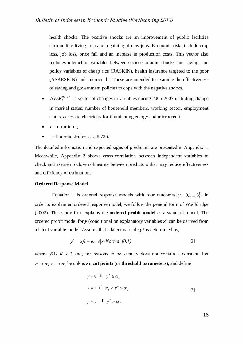
Ordered Response Model
Equation 1 is ordered response models with four outcomes 3,...,1,0y . In
order to explain an ordered response model, we follow the general form of Wooldridge
(2002). This study first explains the ordered probit model as a standard model. The
ordered probit model for y (conditional on explanatory variables x) can be derived from
a latent variable model. Assume that a latent variable y* is determined by,
,* exy xe Normal (0,1) [2]
where is K x 1 and, for reasons to be seen, x does not contain a constant. Let
J ...11be unknown cut points (or threshold parameters), and define
0y if 1
* y
1y if 2
*
1 y [3]
Jy if Jy *

Bulletin of Indonesian Economic Studies (Forthcoming 2013)
19
Given the standard normal assumption for e, the conditional distribution of y given x is
derived straightforward. The computation of each response probability is as below:
xxexPxyPxyP 111
*0
.
.
.
1 122
*
1 xxxyPxyP
[4]
xxxyPxJyP JJJJ 1
*
11
xxyPxJyP JJ 1*
When J=1 we obtain the binary model
111011 xxxyPxyP , and so 1 is the intercept
inside . It is for this reason that x does not contain an intercept in the formulation of
the ordered probit model. The parameters and can be estimated by using
Maximum Likelihood Estimation procedure. For each i, the lod-likelihood function is
iiii xxyxy 121 log11log01,
iJi xJy 1l o g1... [5]
Replacing with the logit function, , will give the ordered logit model. The sign of
estimates coefficients from the ordered probit (logit) models have the exact meaning
with the result of OLS estimations. The negative sign determines whether the choice
probabilities shift to lower categories when the independent variable increases. The
result of estimate coefficients particularly on a partial effect of independent variables,
however, cannot be interpreted directly as the result of Ordinary Least Square (OLS)
estimation. In most cases, we are interested in the response probabilities or partial
effects xjyP of the ordered probit model.
;/ 10 xxxp kk
;/ 1 xxxxp jjkkj [6]
xxxp JkkJ / , Jj 0

Bulletin of Indonesian Economic Studies (Forthcoming 2013)
20
The formula for the response probabilities of the ordered logit model is similar to the
ordered probit model.
This study intended to apply the ordered logit model rather than the ordered
probit model since the distribution of error is assumed following the standard logistic.
The logistic distribution function is similar to the normal distribution function but has a
much simpler form. The ordered logit model in Equation 1 is estimated using three
sample groups: Java-Bali, outside Java-Bali and National (All Sample). Although the
analysis of poverty dynamics focuses on the national level, separating the sample helps
to show the consistency and robustness of estimation results. This also checks whether
there are significant differences of poverty characteristics between Java-Bali and outside
Java-Bali5.
Descriptive Data Analysis
Table 3 shows that households, based on their poverty experience, are divided
into four groups: poor (292 households), transient poor (-) (509 households), transient
poor (+) (769 households) and non-poor (7.156 households). We observed that the poor
group has the following characteristics: they are uneducated or have attained a low
educational attainment; they are living in the rural area, highly dependent on the
agricultural sector (around 80%) and in the informal sector (around 84%); and they
either own a small area of land or are landless households. Compared with the other
groups, the poor group is excluded from modern utility sources. Nearby, 40% of the
poor group does not connect to electricity.
Around 28% of households experienced the negative economic risks and a few
of them has been using saving instruments to cope with these shocks. Daily activities of
poor households are disrupted around 6.4 days/month due to health problems. However,
only a few of them who experienced the negative shocks, either economic risks or
5 This study also wants to estimate the determinants of poverty status (under the lower poverty
line) to check the robustness of regression estimates since the poverty incidence and the
grouping of poverty status are sensitive to the applied poverty line. However, the proportion of
poverty status (under the lower poverty line) to total sample is not representative. At the
national level, the proportions of poor, transient poor (-), transient poor (+) and non-poor are
0.42%, 1.78%, 2.82% and 94.98% respectively. Hence, the regression estimates of determinants
of poverty status (under the lower poverty line) may result biased estimates. Therefore, the
robustness of estimates is checked using three different samples: Java-Bali, Outside Java-Bali
and National.

Bulletin of Indonesian Economic Studies (Forthcoming 2013)
21
health shocks, received government assistance such as the cheap rice (RASKIN) and
health insurance targeted to the poor (ASKESKIN). In the poor group, almost 13% of
households experienced positive shocks of improvement of public facilities in their
surrounding living area. In addition, during 2005-2007, the number of household
members averagely decreased by 0.065 people or almost no change in the number of
household members. Households who are changing in working sectors from agricultural
sectors to non-agricultural sectors and changing in employment status from formal
sectors to informal sectors are both 11.3% on average. Interestingly none of the
households in poor group received microcredit either from the government or from
other sources. They are totally excluded from access to financial services.

Bulletin of Indonesian Economic Studies (Forthcoming 2013)
22
TABLE 3 Descriptive Data of Poverty Status
MeanStd.
Dev.Mean
Std.
Dev.Mean Std. Dev. Mean
Std.
Dev.
Demographic Variables in 2005
1. Marital Status of Household Head (1 = marriage; 0= others) 0.880 0.325 0.853 0.355 0.871 0.335 0.849 0.359
2. Age of Household Head (in years) 47.428 14.281 46.171 14.903 47.429 14.232 45.533 13.709
3. Education Attainment of Household Head (years of schooling) 4.736 3.152 5.096 3.365 5.646 3.191 6.908 4.377
4. Number of Household Member (number of people) 4.719 1.787 4.057 1.744 4.879 1.774 3.853 1.597
5. Dummy of Island (1= Java and Bali; 0= outside Java and Bali) 0.490 0.501 0.477 0.500 0.432 0.496 0.546 0.498
6. Dummy of Location (1= Urban; 0= Rural) 0.045 0.207 0.063 0.243 0.349 0.477 0.463 0.499
Socio-Economic Variables in 2005
7. Working Sector of Household Head (1= agricultural sectors;
0= others)0.805 0.397 0.719 0.450 0.636 0.481 0.446 0.497
8. Employment Status (1= formal sectors; 0= others) 0.158 0.365 0.179 0.384 0.173 0.378 0.303 0.460
9. Land Ownership (in hectare) 0.639 0.789 0.858 1.186 0.737 1.264 0.519 1.593
10. Size of House (in square meter) 59.774 50.192 58.165 27.923 56.671 55.954 70.317 65.373
11. Household with a Family Member Working as Migrant
Workers (TKI) (1= having TKI; 0= others)0.038 0.191 0.043 0.204 0.038 0.191 0.045 0.207
12. Access to Electricity for Illuminating Energy
(1= no access to electricity; 0= having access to electricity)0.390 0.489 0.269 0.444 0.270 0.444 0.100 0.301
Shocks & Risks and Policy Variables in 2005
13. Economic Shocks and Risks (ECSHRS) (1= experiences with
disaster, price falls, crop loss and employment loss;
0= no experiences)
0.284 0.452 0.257 0.438 0.233 0.423 0.158 0.365
14. Cheap Rice (RASKIN) as a Safety Net to Cope with Economic
Shocks and Risks (ECSHRS) (1= experiencing ECSHRS and
receiving RASKIN; 0= others)
0.021 0.142 0.016 0.125 0.027 0.163 0.007 0.083
15. Daily Activities Disrupted by Health Problems for All Family
Members (days in a month)6.363 11.203 4.450 8.607 4.849 8.705 3.729 7.800
16. Insurance to Cope with Health Problems (1= having Health
Insurance Targeted to the Poor (ASKESKIN); 0= others)0.038 0.191 0.028 0.164 0.023 0.151 0.010 0.098
17. Saving as a Coping Strategy to Cope with Economic Risks and
Health Shocks (ECSHRS) (1= having saving; 0= no saving)0.007 0.083 0.006 0.077 0.021 0.143 0.026 0.159
18. Microcredit (1= receiving microcredit; 0= no credit) 0.000 0.000 0.026 0.158 0.016 0.124 0.032 0.177
19. Source of Microcredit (1= government; 0= others) 0.000 0.000 0.008 0.088 0.005 0.072 0.010 0.101
20. Family Member Gaining Employment (1= gaining
employment; 0= others)0.062 0.241 0.045 0.208 0.099 0.299 0.080 0.271
21. Improvement of Public Facilities in Surrounding Living Area
(1= improving public facilities ; 0= others)0.130 0.337 0.092 0.290 0.082 0.274 0.096 0.294
Change Variables during 2005-2007
22. Change in Number of Household -0.065 1.273 0.639 1.502 -0.585 1.672 0.070 1.531
23. Change in Marital Status (1= divorce; 0= others) 0.055 0.228 0.045 0.208 0.062 0.242 0.055 0.229
24. Change in Working Sectors
(1= agricultural sectors to non-agricultural sectors; 0= others)0.113 0.317 0.110 0.313 0.134 0.341 0.140 0.347
25. Change in Employment Status
(1= formal sectors to non-formal sectors; 0= others)0.113 0.317 0.138 0.345 0.081 0.272 0.119 0.324
26. Change in Access to Electricity for Illuminating Energy
(1= gaining access in 2007 but not in 2005; 0= others)0.106 0.309 0.079 0.269 0.131 0.338 0.045 0.206
27. Change in Credits (1= receiving credit in 2007 but not in
2005; 0= others)0.027 0.164 0.037 0.190 0.053 0.225 0.071 0.257
Number of Observation 292 509 769 7,156
Variable
Poor Transient
Poor (-)
Transient
Poor (+)
Non-Poor
Source: Authors’ calculation based on the balanced panel of Susenas 2005 and 2007

Bulletin of Indonesian Economic Studies (Forthcoming 2013)
23
TABLE 4 Descriptive Data used in the Ordered Logit Model
Mean Std. Dev. Mean Std. Dev. Mean Std. Dev.
Demographic Variables in 2005
1. Marital Status of Household Head (1 = marriage; 0= others) 0.850 0.358 0.854 0.353 0.852 0.355
2. Age of Household Head (in years) 46.727 14.030 44.755 13.589 45.801 13.859
3. Education Attainment of Household Head (years of schooling) 6.511 4.265 6.739 4.216 6.618 4.243
4. Number of Household Member (number of people) 3.785 1.538 4.208 1.760 3.984 1.660
5. Dummy of Island (1= Java and Bali; 0= outside Java and Bali) 0.530 0.499
6. Dummy of Location (1= Urban; 0= Rural) 0.506 0.500 0.314 0.464 0.416 0.493
Socio-Economic Variables in 2005
7. Working Sector of Household Head (1= agricultural sectors;
0= others)0.410 0.492 0.581 0.493 0.490 0.500
8. Employment Status (1= formal sectors; 0= others) 0.299 0.458 0.258 0.438 0.280 0.449
9. Land Ownership (in hectare) 0.227 1.091 0.940 1.833 0.562 1.528
10. Size of House (in square meter) 73.383 62.547 62.038 62.368 68.052 62.716
11. Household with a Family Member Working as Migrant
Workers (TKI) (1= having TKI; 0= others)0.042 0.200 0.046 0.209 0.044 0.205
12. Access to Electricity for Illuminating Energy
(1= no access to electricity; 0= having access to electricity)0.027 0.161 0.257 0.437 0.135 0.342
Shocks & Risks and Policy Variables in 2005
13. Economic Shocks and Risks (ECSHRS) (1= experiences with
disaster, price falls, crop loss and employment loss;
0= no experiences)
0.161 0.368 0.190 0.393 0.175 0.380
14. Cheap Rice (RASKIN) as a Safety Net to Cope with Economic
Shocks and Risks (ECSHRS) (1= experiencing ECSHRS and
receiving RASKIN; 0= others)
0.006 0.076 0.014 0.118 0.010 0.098
15. Daily Activities Disrupted by Health Problems for All Family
Members (days in a month)3.737 7.668 4.208 8.527 3.958 8.086
16. Insurance to Cope with Health Problems (1= having Health
Insurance Targeted to the Poor (ASKESKIN); 0= others)0.011 0.104 0.015 0.122 0.013 0.113
17. Saving as a Coping Strategy to Cope with Economic Risks and
Health Shocks (ECSHRS) (1= having saving; 0= no saving)0.027 0.163 0.019 0.137 0.024 0.152
18. Microcredit (1= receiving microcredit; 0= no credit) 0.046 0.209 0.011 0.104 0.029 0.169
19. Source of Microcredit (1= government; 0= others) 0.016 0.125 0.002 0.044 0.009 0.096
20. Family Member Gaining Employment (1= gainin employment;
0= others)0.082 0.274 0.075 0.264 0.079 0.269
21. Improvement of Public Facilities in Surrounding Living Area
(1= improving public facilities; 0= others)0.102 0.303 0.088 0.283 0.095 0.294
Change Variables during 2005-2007
22. Change in Number of Household 0.071 1.416 0.007 1.693 0.041 1.553
23. Change in Marital Status (1= divorce; 0= others) 0.049 0.216 0.063 0.242 0.055 0.229
24. Change in Working Sectors
(1= agricultural sectors to non-agricultural sectors; 0= others)0.136 0.343 0.138 0.345 0.137 0.344
25. Change in Employment Status
(1= formal sectors to non-formal sectors; 0= others)0.117 0.322 0.116 0.320 0.117 0.321
26. Change in Access to Electricity for Illuminating Energy
(1= Gaining access in 2007 but not in 2005; 0= others)0.016 0.127 0.101 0.302 0.056 0.230
27. Change in Credits (1= receiving credit in 2007 but not in 2005; 0= others) 0.080 0.272 0.050 0.218 0.066 0.248
Poverty Status
Poor
Transient Poor (-)
Transient Poor (+)
Non-Poor
Number of Observation
292143 149
8,726
Variable
Java and Bali Outside
Java and Bali
4,626 4,100
National
509
769
7,156
243
332
3,908
266
437
3,248
Source: Authors’ calculation based on the balanced panel of Susenas 2005 and 2007

Bulletin of Indonesian Economic Studies (Forthcoming 2013)
24
In the case of the transient poor (-) group, the demographic characteristics and
socio-economic variables are slightly better than those of the poor group. This group has
higher educational attainment, better access to electricity and owns larger areas of land
(0.86 hectare). Households experiencing economic risks and health shocks are lower
than poor group. Daily activities disrupted by health shocks are two days lower than the
poor group. This study finds that the major variable changes faced by the transient (-)
group during 2005-2007 was an increase of one household member, change in
employment status from formal sectors to the informal sector (14%).
In contrast to the transient poor (-) group, the transient poor (+) group has
mostly completed elementary school, lives in an urban area (35%), has better access to
electricity, has a low percentage working in agricultural sectors, has a low percentage of
households experiencing economic and health risks and has sufficient savings to cope
with economic and health risks. The greatest difference between the transient (+) group
and the two previous groups is a decrease of almost one household members, a larger
proportion of households receiving microcredit, a higher proportion of households
gaining access to electricity and a low percentage of households moving from formal
sectors to informal sectors.
Lastly, the non-poor group has different characteristics compared to the other
three groups. They are more educated households, with almost the majority having
completed junior high school; they have fewer household members, live in urban area;
they have a better connection to electricity (90%), less experience of economic risks and
health shocks and have enough savings to cope with negative shocks. The daily
activities of households in this group are disrupted by health shocks only 3.7 days in a
month, around half of that experienced by the poor group. Furthermore, they are
working in formal sectors and non-agricultural sectors so the income is less volatile and
does not depend on assistance from the government.
Table 4 shows that households, based on the living location, are divided into
three sub groups: Java-Bali (53%), outside Java-Bali (47%) and National. Households
living in Java-Bali could be classified as poor (3.1%), transient poor (-) (5.25%),
transient poor (+) (7.18%) and non-poor (84.48%). Households living outside Java-Bali
could be classified as poor (3.63%), transient poor (-) (6.49%), transient poor (+)
(10.66%) and non-poor (79.22%). These figure show that households outside Java-Bali
Bulletin of Indonesian Economic Studies (Forthcoming 2013)
25
are more vulnerable to being transient poor, both (-) and (+), compared to households in
Java-Bali.
The significant differences between households living in Java-Bali and outside
Java-Bali are that households outside Java-Bali have more family members (4.2 people),
mostly live in a rural area (69%) and have a wider agricultural land (almost 1 hectare).
Almost 97% households in Java-Bali are connected to electricity while only 74%
households outside Java-Bali have electricity connections for their sources of
illuminating energy. Furthermore, households outside Java-Bali experienced more
economic risks and health shocks than households in Java-Bali. Around 19% of
household outside Java-Bali experienced economic risks and shocks while only 16% of
households in Java-Bali experienced them. Daily activities of households outside
Java-Bali are disturbed a half day more than households in Java-Bali due to health
shocks.
THE DETERMINANTS OF POVERTY DYNAMICS IN INDONESIA
This study estimated three models: Java-Bali (MODEL 1), Outside Java-Bali
(MODEL 2) and National (MODEL 3). The aim of separating the sample is to ensure
the consistency and robustness of estimation. The models are estimated using the
maximum likelihood estimation with robust standard errors. The estimation results of
the ordered logit model are shown in Table 5 and Table 6. The signs of coefficients in
the three models are almost the same except in the following variables: age of
household head (outside Java-Bali), economic shocks and risks (outside Java-Bali),
source of microcredits (outside Java-Bali) and change in marital status (Java-Bali). All
models show that the Wald Chi-Square statistics of Log likelihood of ordered logit
model are statistically significant indicating at least one of the covariates or independent
variables affects the poverty status of households. Generally, the built ordered logit
models of the poverty dynamics show their consistency and robustness.
The Pseudo R-squared ranges from 11.05% to 14.62%. These values seem too
small but are often found in household data analysis either using OLS or a non-linear
model, i.e. discrete choice model or categorical outcome variables due to a larger

Bulletin of Indonesian Economic Studies (Forthcoming 2013)
26
variation on household data6. Another possible reason for the low value of Pseudo
R-squared on these estimates is that most predictors (independent variables) are dummy
variables (not continuous variables) so it will not improve greatly the log likelihood.
The Pseudo R-squared of many studies on poverty dynamics is also ranging from 19%
(Alisjahbana and Yusuf, 2003), 10% and 26.46% (Cruces and Wodon, 2003), and 7.87%
and 14.00% (McCulloch and Calandrino, 2003).
Table 6 shows the partial effects (dy/dx) of changes in a probability of
households being poor, transient poor (-), transient poor (+) and non-poor responding to
change in independent variables (predictors). The partial effects (the predicted
probability of household poverty status) evaluated at means of independent variables
xjy . The probability of households in Java-Bali being poor, transient poor (-),
transient poor (+) and non-poor are 1.5%, 3.2%, 5.4% and 89.9% respectively. On the
other hand, the probability of households outside Java-Bali being poor, transient poor (-),
transient poor (+) and non-poor are 2.2%, 4.7%, 9.5% and 83.6% respectively. If the
household characteristics are the same as the average value of the sample, the
probability of households being non-poor is almost 90% in Java-Bali and 84% outside
Java-Bali while the probability of households being poor is 1.5% in Java-Bali and 2.2%
outside Java-Bali. Furthermore, households living outside Java-Bali have a higher
probability of being either transient poor (-) or transient poor (+) than households living
in Java-Bali.
Demographic Variables
All models statistically confirmed the demographic variables such as the
number of household members, educational attainment (years of schooling) and location
are the important factors in distinguishing the poverty status of households. In addition,
6 The evaluation of the goodness of fit of logistic regression (discrete outcome variables) is
evaluated based on Pseudo R2 with the higher value indicating a better model fit. One approach
of calculating Pseudo R2 adapted by the STATA software package is McFadden’s mirror
approaches 1 and 2. McFadden Approach and McFadden Approach Adjusted are
.
2
ˆln
ˆln1
Inc
full
ML
MLR and
.
2
ˆln
ˆln1
Inc
full
ML
KMLR
, respectively; where L̂ is estimated
likelihood; fullM is model with predictors; .incM is model without predictors (only intercept)
and K is number of predictors.
Bulletin of Indonesian Economic Studies (Forthcoming 2013)
27
the variables of marital status and age of the household head are both statistically
significant influencing the poverty status at a national level (MODEL 3) but not in
MODEL 1 (Marital Status) and MODEL 2 (Age). Married households outside Java-Bali
have a higher probability being non-poor. This is because most of the households
outside Java-Bali are working in the agricultural sectors, labour intensive; so a married
household has more labour supply to produce more outputs or incomes than a single
household.
Table 6 shows an increase in number of household member decrease the
probability of being non-poor by 4.6% while this increases the probability being poor,
transient poor (-) and transient poor (+) by 0.8%, 1.5% and 2.4% respectively (MODEL
3). This finding is similar to Herrera (1999), Haddad and Ahmed (2003), Woolard and
Klasen (2005). Given a fixed income, an increase in the number of members forced the
households to reduce their consumption and to support the additional member(s).
Meanwhile, a better education raises the probability of being non-poor because a
higher-education level provides a higher opportunity for a better job and higher income.
These findings confirmed the conclusions of other studies such as Adam and Jane
(1995), Jalan and Ravallion (1998), McCulloch and Baulch (2000), Alisjahbana and
Yusuf (2003), Bigsten et al. (2003), Mango et al. (2004), and Widyanti et al. (2009).
Dummy of location has an ability to distinguish the poverty status of
households in three models. Those living in urban areas have a higher probability of
being non-poor. These findings of location dummy significantly influencing the poverty
status in Indonesia confirmed other study findings in countries such as Bigsten et al.
(2003), Fields et al. (2003), Okidi and McKay (2003) and Kedir and McKay (2005).
Urban areas where most industries and economic activities are located provide more job
opportunities either in the formal or informal sector.
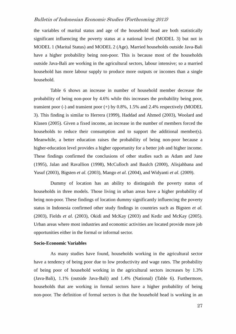
Socio-Economic Variables
As many studies have found, households working in the agricultural sector
have a tendency of being poor due to low productivity and wage rates. The probability
of being poor of household working in the agricultural sectors increases by 1.3%
(Java-Bali), 1.1% (outside Java-Bali) and 1.4% (National) (Table 6). Furthermore,
households that are working in formal sectors have a higher probability of being
non-poor. The definition of formal sectors is that the household head is working in an

Bulletin of Indonesian Economic Studies (Forthcoming 2013)
28
agency/office/company with a fixed salary either in cash or in goods. Those working in
formal sectors increase their probability of being non-poor by 5.8% (National), 6.8%
(outside Java-Bali) and 4.6% (Java-Bali). This is because formal sectors guarantee a
stable income and pay higher wage rates than the informal sectors. Kedir and McKay
(2005) also confirmed that those who are working as waged employees have a better
probability to escape from poverty in Rural Ethiopia.
On the other hand, because of the lack of job opportunities in Indonesia,
individuals who could not find jobs in the formal sectors and start a business
(entrepreneur) are forced to either work in domestic informal sectors with a low wage
rate or to work outside Indonesia as migrant workers. Most migrant workers are also
working in informal sectors as domestic helpers, but they are paid a higher wage rate.
This study confirmed that households having a family member working outside
Indonesia tend to be non-poor due to remittances that can form either family transfers to
support basic needs or entrepreneur capital transfers to support their families to start up
a business. Hall (2007) also showed remittances have an important role in the poverty
dynamics in Latin America. This variable, however, is insignificant in the sample of
outside Java-Bali.
Land ownership as an indicator of physical assets significantly affects the
poverty status of households. Three models show that one hectare increase in land will
increase the probability of being non-poor between 1.6% (Java-Bali), 1.3% (outside
Java-Bali) and 1.7% (National). Landless and small landholder households tend to be
chronic poor since their productive assets are inadequate to increase their income. Land
reforms to increase the ownership of productive assets of poor households should be
considered as a policy alternative to alleviate chronic poverty. This finding is similar to
the discoveries of Adam and Jane (1995), Jalan and Ravallion (1998), McCulloch and
Baulch (2000), Haddad and Ahmed (2003), and Woolard and Klasen (2005). The size of
a house as one indicator of physical assets can also determine the poverty status of
households. A larger size of a house will increase the probability of being non-poor.
Both findings imply that certification of agricultural land and house ownership is among
possible policy alternatives to alleviate poverty. The certification would legalize land
and house ownership that could be utilized as collateral for gaining productive credit
from the formal institution.
Bulletin of Indonesian Economic Studies (Forthcoming 2013)
29
Other socio-economic variables such as access to modern utilities of electricity
significantly increase a probability to climb out of poverty. The unit cost of lighting
with electricity is cheaper per kilowatt-hour than lighting with candles or oil lamp.
Therefore, households can save energy expenditure that can potentially be reallocated to
income-generating activities or, in the case of children, to education. This can ultimately
serve to free households from poverty. Table 4 shows that households in Java-Bali have
better access to electricity than households outside Java-Bali due to a better availability
of electricity grid. A lack of access to electricity of households outside Java-Bali is more
due to a lack of availability of electricity grid rather than the inability of the household
to pay a connection fee (LPEM FEUI, PSE-KPUGM, PSP-IPB, 2004b). Thus, the
government should widen access to electricity especially for households outside
Java-Bali as one of its poverty alleviation policies.
Shocks, Risks and Government Assistance
Low income groups in most developing countries usually face volatility in
consumption due to external shocks, either positive or negative. Dartanto and Nurkholis
(2010) found that households in a rural area of Kebumen, Indonesia are vulnerable from
negative shocks and they will respond differently to negative shocks depending on
consumption structure, asset ownership, cattle ownership and family assistance.
Interestingly, this study found that there are significant differences in
behaviours between households living in Java-Bali and outside Java-Bali responding to
economic risks and health shocks. Households living in Java-Bali are more vulnerable
to negative shocks while households living outside Java-Bali are relatively resilient to
negative shocks. Even so, households outside Java-Bali experienced more negative
shocks than households in Java-Bali (Table 4) but the estimation results showed that the
coefficients of economic risks and health shocks are statistically insignificant affecting
the poverty status of households outside Java-Bali. This might be due to households
outside Java-Bali generally working in agricultural sectors and owning larger lands.
They, therefore, could reduce agricultural risks such as crop loss and price fall through a
diversification in agricultural cultivations.

Bulletin of Indonesian Economic Studies (Forthcoming 2013)
30
TABLE 5 Estimation Results of Ordered Logit Model
Coeff. Robust
Std. Error
Coeff. Robust
Std. Error
Coeff. Robust
Std. Error
Demographic Variables in 2005
1. Marital Status of Household Head (1 = marriage; 0= others) 0.198 0.145 0.295 0.134** 0.239 0.097***
2. Age of Household Head (in years) -0.007 0.004* 0.004 0.004 -0.002 0.003***
3. Education Attainment of Household Head (years of schooling) 0.079 0.012*** 0.052 0.011*** 0.068 0.008***
4. Number of Household Member (number of people) -0.431 0.032*** -0.421 0.028*** -0.402 0.021***
5. Dummy of Island (1= Java and Bali; 0= outside Java and Bali) -0.410 0.073***
6. Dummy of Location (1= Urban; 0= Rural) 1.283 0.105*** 0.291 0.115** 0.868 0.079***
Socio-Economic Variables in 2005
7. Working Sector of Household Head (1= agricultural sectors; 0= others) -0.822 0.109*** -0.540 0.113*** -0.720 0.077***
8. Employment Status (1= formal sectors; 0= others) 0.544 0.161*** 0.544 0.161*** 0.544 0.113***
9. Land Ownership (in hectare) 0.182 0.091** 0.095 0.033*** 0.149 0.032***
10. Size of House (in square meter) 0.006 0.002*** 0.007 0.003** 0.006 0.002***
11. Household with a Family Member Working as Migrant
Workers (TKI) (1= having TKI; 0= others)0.716 0.247*** 0.097 0.219 0.337 0.159**
12. Access to Electricity for Illuminating Energy
(1= no access to electricity; 0= having access to electricity)-1.984 0.290*** -1.033 0.124*** -0.916 0.108***
Shocks & Risks and Policy Variables in 2005
13. Economic Shocks and Risks (ECSHRS) (1= experiencing with disaster,
price falls, crop loss and employment loss; 0= no experiences)-0.377 0.111*** 0.005 0.114 -0.173 0.079**
14. Cheap Rice (RASKIN) as a Safety Net to Cope with Economic Shocks
and Risks (ECSHRS) (1= experiencing ECSHRS and receiving RASKIN;
0= others)
-0.241 0.378 -0.204 0.282 -0.107 0.229
15. Daily Activities Disrupted by Health Problems for All Family
Members (days in a month)-0.010 0.005** -0.007 0.005 -0.007 0.004*
16. Insurance to Cope with Health Problems (1= having Health Insurance
Targeted to the Poor (ASKESKIN); 0= others)-1.164 0.280*** -0.337 0.307 -0.646 0.212***
MODEL 2:
Outside
Java and Bali
MODEL 3:
National
Variable
MODEL 1:
Java and Bali

Bulletin of Indonesian Economic Studies (Forthcoming 2013)
31
TABLE 5 Estimation Results of Ordered Logit Model (Continued)
Coeff. Robust
Std. Error
Coeff. Robust
Std. Error
Coeff. Robust
Std. Error
Shocks & Risks and Policy Variables in 2005 (Continued)
17. Saving as Coping Strategy to Cope with Economic Risks and
Health Shocks (1= having saving; 0= no saving)0.558 0.309* 0.653 0.368* 0.596 0.243***
18. Microcredit (1= receiving microcredit; 0= no credit) 0.920 0.382** 0.118 0.400 0.639 0.278**
19. Source of Microcredit (1= government; 0= others) -0.254 0.608 0.475 1.049 0.085 0.492
20. Family Member Gaining Employment (1= gaining employment;
0= others)0.364 0.173** 0.062 0.156 0.219 0.115*
21. Improvement of Public Facilities in Surrounding Living Area
(1= improving public facilities; 0= others)-0.318 0.136** 0.601 0.178*** 0.092 0.108
Change Variables during 2005-2007
22. Change in Number of Household -0.152 0.031*** -0.184 0.026*** -0.160 0.020***
23. Change in Marital Status (1= divorce; 0= others) 0.048 0.218 -0.342 0.176** -0.190 0.135
24. Change in Working Sectors
(1= agricultural sectors to non-agricultural sectors; 0= others)0.528 0.148*** 0.240 0.129* 0.393 0.096***
25. Change in Employment Status
(1= formal sectors to non-formal sectors; 0= others)-0.265 0.213 -0.675 0.194*** -0.500 0.141***
26. Change in Access to Electricity for Illuminating Energy
(1= getting access in 2007 but not in 2005; 0= others)1.318 0.356*** 0.151 0.137 0.150 0.128
27. Change in Credits (1= receiving credit in 2007 but not in 2005; 0= others) 0.431 0.179** 0.826 0.237*** 0.531 0.138***
/cut0 -4.510 0.289*** -4.614 0.275*** -4.631 0.200***
/cut1 -3.327 0.288*** -3.430 0.270*** -3.465 0.197***
/cut2 -2.496 0.282*** -2.460 0.265*** -2.576 0.193***
Number of Observation
Log Pseudolikelihood
Wald Chi-Squared
Pseudo R-Squared
1,102.26
0.1170
561.21
0.1105
Variable
MODEL 1:
Java and Bali
MODEL 2:
Outside
Java and Bali
MODEL 3:
National
-5,055.63-2,345.27
708.78
0.1462
4,100
-2,629.68
4,626 8,726
Source: Authors’ Estimates. *, **, *** are significant at 10%, 5% and 1% respectively.

Bulletin of Indonesian Economic Studies (Forthcoming 2013)
32
Households in Java-Bali experiencing economic risks resulting from crop loss,
job loss and price falls have a tendency to be poor and transient poor. Moreover, health
shocks represented by a number of daily activities disrupted by health problems are
significantly affecting the poverty status of households. Those experiencing these
shocks tend to be poor. This finding is consistent with Contreras et al. (2004) in Chile.
However, three models confirmed households experiencing either economic or health
shocks and having enough savings should be able to cope with these shocks easily and
to keep their poverty status as non-poor household. MODEL 3 shows that having
savings will decrease the probability of being poor and transient poor (-) by 0.9% and
1.7% respectively (MODEL 3).
This study includes only four types of government assistance: cheap rice
(RASKIN), health insurance targeted to the poor (ASKESKIN), microcredit and
improvement of public facilities due to data availability in the Susenas panel dataset and
considering the relation with shocks. Even so, the interaction variable of cheap rice
(RASKIN) and economic shocks and risks (ECSHRS) does not statistically affect the
poverty status of households but the probability of households being poor decreases
from 0.6% to 0.4% when the government distributed cheap rice to households in
Java-Bali who are experiencing economic risks and shocks (ECSHRS). This study
confirmed Sumarto et al.’s (2005) findings that the subsidized rice programme appears
to reduce the risk of poverty. Further, the probabilities of being poor and transient poor
(-) for those who are experiencing health shocks and receiving ASKESKIN in Java-Bali
are 3.1% and 5.7% correspondingly.
Unexpected results that statistical evidences do not confirm the effectiveness of
both policies to protect the poor might be due to wrong targets and uneven distribution
of government assistance as indicated in Table 3 and Table 4. The proportions of
households experiencing health problems and receiving health insurance targeted for the
poor (ASKESKIN) are 3.8% of the poor group, 2.8% of the transient poor (-) group,
2.3% of the transient poor (+) group and 1% of the non-poor group. Similar proportions
are also found in the case of households experiencing economic shocks and risks
(ECSHRS) and receiving cheap rice (RASKIN). Approximately 7.4% of poor
households that experienced economic shocks and risks received cheap rice (RASKIN).
At the disaggregate regional level, the proportions of government assistance (RASKIN
and ASKESKIN) received by households experiencing economic shocks, risks and

Bulletin of Indonesian Economic Studies (Forthcoming 2013)
33
health shocks are also relatively small. These facts should encourage the government to
improve the distribution of assistance. The government should not only focus on
providing assistance based on the poverty condition but also pay attention to such
shocks/events experienced by households.
On the contrary, microcredit is well functioned as a poverty alleviation
programme, particularly in Java-Bali. This may simply reflect households living in
Java-Bali have better access to this programme. The proportion of households receiving
microcredit in Java-Bali is 4.6% while only 1.1% of households living outside Java-Bali
received this programme. The positive coefficient of microcredit in all three models
marks that households receiving credit programmes tend to be non-poor. Microcredit
either coming from the government or from others is not necessary related to the
poverty status. This finding confirmed that microcredit has an important role in
alleviating poverty in Indonesia. Deploying accesses to either microcredit or financial
institutions particularly outside Java-Bali might significantly speed up the poverty
reduction in this area. Moreover, the positive shock of obtaining jobs improves the
poverty status of households. Gaining an employment is identical with increased
income or expenditure in that both can lift the household from poverty. If a household
member can find a job, the probability of being poor in Java-Bali and nationally will
decrease by 0.5% and 0.4% respectively. This confirmed Fields et al.’s (2003) findings
that gaining a job would lift the household out of poverty in Indonesia.
In addition, the improvement of public facilities such as the development of
bridges and roads has a positive effect on poverty alleviation, particularly outside
Java-Bali where these regions often face infrastructure bottlenecks. The probability of
households being non-poor outside Java-Bali increases by 6.9% along with the
development of public facilities in this area. In contrast to the finding outside Java-Bali,
the estimation result is quite surprising in that infrastructure developments in Java-Bali
do not have a positive impact on improving the poverty status. This is most likely
because Java-Bali is a well-developed region that already had good infrastructures. Thus,
new constructions such as toll roads sometimes lead to either land acquisitions or
eviction of residents. Another example, the renovation of traditional markets into
modern markets occasionally marginalizes previous traders because of their inability to
afford the new price of buildings. These conditions might send households living in
Java-Bali into poverty.

Bulletin of Indonesian Economic Studies (Forthcoming 2013)
34
Changes in Household Indicators during 2005-2007
Lastly, this part discusses the impact on poverty status of some changes in
demographic, socio-economic and government assistance variables during 2005 to 2007.
An increase of one family member decreases the probability of the household being
non-poor by 1.9% at a national level. An increase of one family member is associated
with falling into poverty since a given amount of resources needs to be redistributed to
support the new member. Households with a high dependent ratio could not save and
allocate the resources into other productive activities to assist them in moving out of the
poverty. This finding should encourage government at any level to continuously and
actively promote a family planning programme. Change in the demographic variable of
marital status due to divorce is also positively increasing the probability of households
being poor and transient poor (-) outside Java-Bali but not in Java-Bali. A divorce
results in the loss of productive family members, either the mother or father that might
reduce household ability and capacity in terms of economic power. This is consistent
with Woolard and Klasen’s (2005) finding that female headed households tend to fall
into poverty in South Africa.
Further, change in working status from an agricultural to a non-agricultural
sector increases the probability of households being non-poor. Non-agricultural sectors
theoretically pay higher and more stable wage rates. Therefore, households are able to
increase and smooth their consumption level. Those who are able to find a job in a
non-agricultural sector will increase their probability of being non-poor by 4.1%
(Java-Bali), 3.1% (outside Java-Bali) and 4.1% (National). A structural reform through
either changing the economic basis from agriculture into non-agriculture or changing
traditional agriculture into an agriculture-based industry should be considered as an
important policy to alleviate poverty. Meanwhile, a change in employment status from
the formal sector into the informal sector sends a previously non-poor household into
poverty. Households experiencing layoffs and finding new jobs either as an employee or
as self-employment in informal sectors is associated with a higher probability of being
either poor or transient poor (-). Those experiencing layoffs and finding new jobs in the
informal sector will decrease their probability of being non-poor by 6.6% at a national
level.
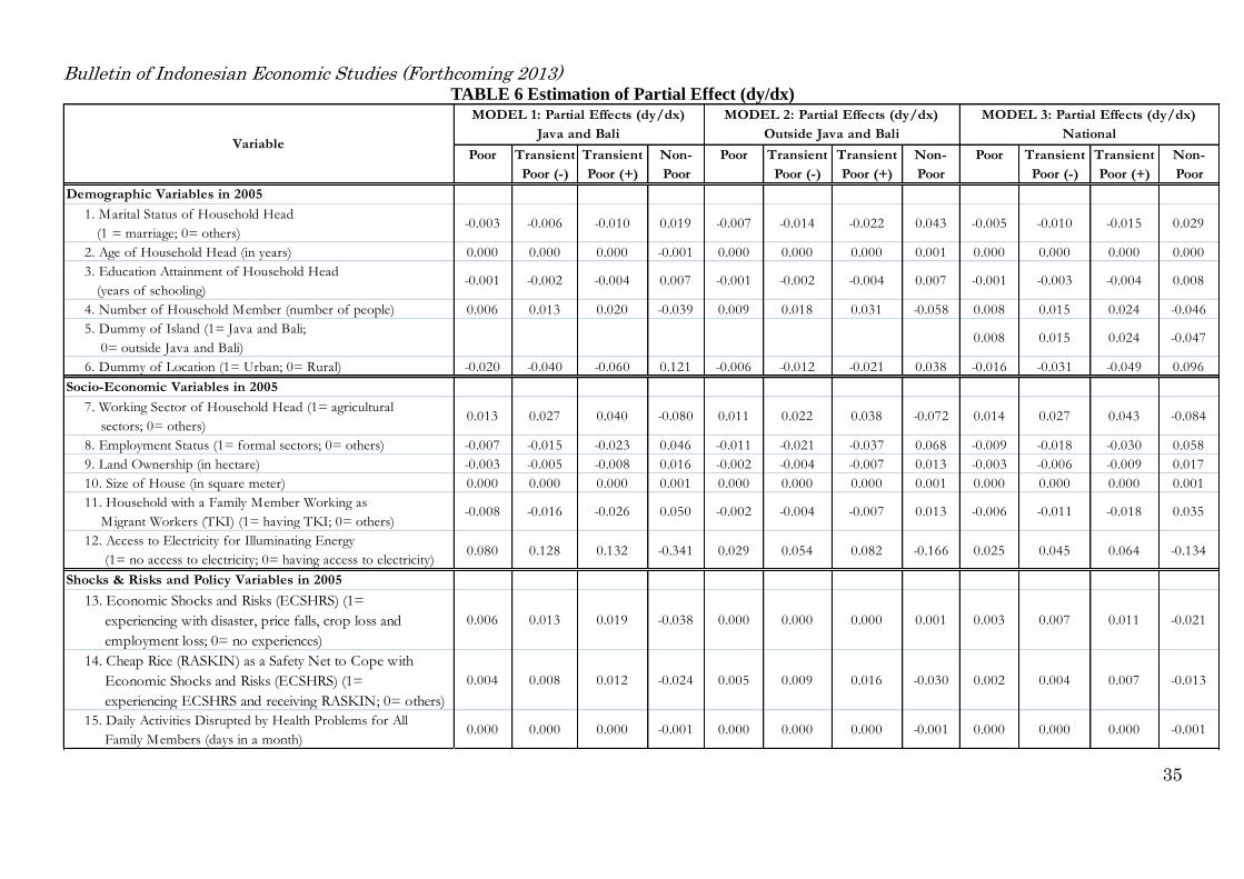
Bulletin of Indonesian Economic Studies (Forthcoming 2013)
35
TABLE 6 Estimation of Partial Effect (dy/dx)
Poor Transient
Poor (-)
Transient
Poor (+)
Non-
Poor
Poor Transient
Poor (-)
Transient
Poor (+)
Non-
Poor
Poor Transient
Poor (-)
Transient
Poor (+)
Non-
Poor
Demographic Variables in 2005
1. Marital Status of Household Head
(1 = marriage; 0= others)-0.003 -0.006 -0.010 0.019 -0.007 -0.014 -0.022 0.043 -0.005 -0.010 -0.015 0.029
2. Age of Household Head (in years) 0.000 0.000 0.000 -0.001 0.000 0.000 0.000 0.001 0.000 0.000 0.000 0.000
3. Education Attainment of Household Head
(years of schooling)-0.001 -0.002 -0.004 0.007 -0.001 -0.002 -0.004 0.007 -0.001 -0.003 -0.004 0.008
4. Number of Household Member (number of people) 0.006 0.013 0.020 -0.039 0.009 0.018 0.031 -0.058 0.008 0.015 0.024 -0.046
5. Dummy of Island (1= Java and Bali;
0= outside Java and Bali)0.008 0.015 0.024 -0.047
6. Dummy of Location (1= Urban; 0= Rural) -0.020 -0.040 -0.060 0.121 -0.006 -0.012 -0.021 0.038 -0.016 -0.031 -0.049 0.096
Socio-Economic Variables in 2005
7. Working Sector of Household Head (1= agricultural
sectors; 0= others)0.013 0.027 0.040 -0.080 0.011 0.022 0.038 -0.072 0.014 0.027 0.043 -0.084
8. Employment Status (1= formal sectors; 0= others) -0.007 -0.015 -0.023 0.046 -0.011 -0.021 -0.037 0.068 -0.009 -0.018 -0.030 0.058
9. Land Ownership (in hectare) -0.003 -0.005 -0.008 0.016 -0.002 -0.004 -0.007 0.013 -0.003 -0.006 -0.009 0.017
10. Size of House (in square meter) 0.000 0.000 0.000 0.001 0.000 0.000 0.000 0.001 0.000 0.000 0.000 0.001
11. Household with a Family Member Working as
Migrant Workers (TKI) (1= having TKI; 0= others)-0.008 -0.016 -0.026 0.050 -0.002 -0.004 -0.007 0.013 -0.006 -0.011 -0.018 0.035
12. Access to Electricity for Illuminating Energy
(1= no access to electricity; 0= having access to electricity)0.080 0.128 0.132 -0.341 0.029 0.054 0.082 -0.166 0.025 0.045 0.064 -0.134
Shocks & Risks and Policy Variables in 2005
13. Economic Shocks and Risks (ECSHRS) (1=
experiencing with disaster, price falls, crop loss and
employment loss; 0= no experiences)
0.006 0.013 0.019 -0.038 0.000 0.000 0.000 0.001 0.003 0.007 0.011 -0.021
14. Cheap Rice (RASKIN) as a Safety Net to Cope with
Economic Shocks and Risks (ECSHRS) (1=
experiencing ECSHRS and receiving RASKIN; 0= others)
0.004 0.008 0.012 -0.024 0.005 0.009 0.016 -0.030 0.002 0.004 0.007 -0.013
15. Daily Activities Disrupted by Health Problems for All
Family Members (days in a month)0.000 0.000 0.000 -0.001 0.000 0.000 0.000 -0.001 0.000 0.000 0.000 -0.001
MODEL 3: Partial Effects (dy/dx)
NationalVariable
MODEL 1: Partial Effects (dy/dx)
Java and Bali
MODEL 2: Partial Effects (dy/dx)
Outside Java and Bali

Bulletin of Indonesian Economic Studies (Forthcoming 2013)
36
TABLE 6 Estimation of Partial Effect (dy/dx) (Continued)
Poor Transient
Poor (-)
Transient
Poor (+)
Non-
Poor
Poor Transient
Poor (-)
Transient
Poor (+)
Non-
Poor
Poor Transient
Poor (-)
Transient
Poor (+)
Non-
Poor
Shocks & Risks and Policy Variables in 2005 (Continued)
16. Insurance to Cope with Health Problems (1= having
Health Insurance Targeted to the Poor (ASKESKIN);
0= others)
0.031 0.057 0.074 -0.162 0.009 0.016 0.026 -0.051 0.017 0.031 0.045 -0.093
17. Saving as Coping Strategy to Cope with Economic Risks
and Health Shocks (1= having saving; 0= no saving)-0.006 -0.013 -0.021 0.041 -0.011 -0.022 -0.040 0.072 -0.009 -0.017 -0.030 0.056
18. Microcredit (1= receiving microcredit; 0= no credit) -0.009 -0.019 -0.032 0.060 -0.002 -0.005 -0.008 0.016 -0.009 -0.018 -0.031 0.059
19. Source of Microcredit (1= government; 0= others) 0.004 0.008 0.013 -0.025 -0.008 -0.017 -0.030 0.055 -0.002 -0.003 -0.005 0.009
20. Family Member gaining employment
(1= gaining employment; 0= others)-0.005 -0.010 -0.015 0.029 -0.001 -0.003 -0.004 0.008 -0.004 -0.007 -0.012 0.024
21. Improvement of Public Facilities in Surrounding
Living Area (1= improving public facilities; 0= others)0.005 0.011 0.016 -0.032 -0.010 -0.021 -0.038 0.069 -0.002 -0.003 -0.005 0.010
Change Variables during 2005-2007
22. Change in Number of Household 0.002 0.005 0.007 -0.014 0.004 0.008 0.013 -0.025 0.003 0.006 0.010 -0.019
23. Change in Marital Status (1= divorce; 0= others) -0.001 -0.001 -0.002 0.004 0.009 0.016 0.027 -0.052 0.004 0.008 0.012 -0.023
24. Change in Working Sectors (1= agricultural sectors
to non-agricultural sectors; 0= others)-0.006 -0.013 -0.021 0.041 -0.005 -0.010 -0.017 0.031 -0.007 -0.013 -0.021 0.041
25. Change in Employment Status
(1= formal sectors to non-formal sectors; 0= others)0.004 0.009 0.013 -0.026 0.019 0.035 0.054 -0.109 0.011 0.022 0.033 -0.066
26. Change in Access to Electricity for Illuminating Energy
(1= gaining access in 2007 but not in 2005;
0= others)
-0.011 -0.023 -0.039 0.073 -0.003 -0.006 -0.011 0.020 -0.003 -0.005 -0.009 0.017
27. Change in Credits (1= receiving credit in 2007
but not in 2005; 0= others)-0.005 -0.011 -0.018 0.034 -0.013 -0.026 -0.048 0.087 -0.008 -0.016 -0.027 0.052
Probability (y = j |x) 0.015 0.032 0.054 0.899 0.022 0.047 0.095 0.836 0.019 0.040 0.074 0.867
MODEL 1: Partial Effects (dy/dx)
Java and Bali
MODEL 2: Partial Effects (dy/dx)
Outside Java and Bali
MODEL 3: Partial Effects (dy/dx)
NationalVariable
Source: Authors’ estimation
Note: dy/dx is for discrete change of dummy variable from 0 to 1

Bulletin of Indonesian Economic Studies (Forthcoming 2013)
37
The role of infrastructure development such as widening access to electricity in
Indonesia is clearly confirmed by MODEL 1. Expanding electricity access to poor
households will decrease the probability of being poor in Java-Bali by 1.1%. Increasing
access to electricity can substantially enhance the productivity of households and
household based micro-enterprises. Electricity makes possible the use of appliances that
substantially increase productivity and hence the income generating potential of
micro-enterprises (pumps, sewing machines, power tools), while information and
communication technologies enhance the availability of market information and the
possibility of social and political participation (LPEM FEUI, PSE-UGM, PSP-IPB,
2004a and 2004b).
Among the most interesting finding related to the changes of government
assistance is that the poor group obtaining credit programmes are able to improve their
standard of living and climb out of the poverty. The programme enables and equips
households to start up small businesses, create job opportunities, and empower
themselves. At the end, this enables them to move out from the poverty. Households
receiving microcredit during 2005-2007 will increase their probability of being
non-poor by 3.4% (Java-Bali), 8.7% (outside Java-Bali) and 5.2% (National).
Expanding microcredit, particularly outside Java-Bali where financial institutions have
not developed well yet, will accelerate the poverty reduction in Indonesia.
CONCLUDING REMARKS
Observing the Susenas panel dataset of 2005 and 2007 and applying the spell
approach in determining poverty status of households, we found that around 28% of
poor households in Indonesia could be considered as chronic poor (remained poor in
two periods) and roughly 7% of non-poor households is vulnerable to being transient
poor (-). Poverty in Indonesia is a rural phenomenon and quite sensitive to change in the
poverty line. A 25% increase in the poverty line causes more than a two-fold increase in
the poverty rate. Further, the rural households are more vulnerable to falling into
poverty than urban households. During 2005-2007, around 11% of rural non-poor
households fell into poverty while only 1% of 2005 urban non-poor households did.
Around 30% of poor households in Java-Bali and around 25% of poor households
outside Java-Bali are categorized as poor (poor in two periods) households. Further,

Bulletin of Indonesian Economic Studies (Forthcoming 2013)
38
outside Java-Bali contributed more in transient poor while Java-Bali contributed more
in poor (chronically or remained poor in two periods).
This study applying the ordered logit model found that the important factors of
poverty dynamics in Indonesia are educational attainment, the number of household
member, physical assets (land and house ownership), working sector, employment
status, access to modern utilities of electricity, changes in the household size, in the
working sector, in the employment status, and in the microcredit programme. The
estimation of partial effects of change in independent variables confirmed that one
hectare increase in land will increase the probability of being non-poor between 1.6%
(Java-Bali), 1.3% (outside Java-Bali) and 1.7% (National). An increase of one family
member decreases the probability of the household being non-poor by 1.9% (national).
Besides, households receiving microcredit during 2005-2007 will increase their
probability of being non-poor by 3.4% (Java-Bali), 8.7% (outside Java-Bali) and 5.2%
(National).
This study also found the interesting findings that households living in
Java-Bali are more vulnerable to negative shocks while households living outside
Java-Bali are relatively resilience to negative shocks. Moreover, no consistent statistical
evidence in three models supports the hypothesis that the role of government policies
such as cheap rice (RASKIN) and health insurance targeted to the poor (ASKESKIN) as
an instrument to cope with negative shocks. Microcredit programmes, however, are well
functioned as a poverty alleviation policy. Even though, there is no consistent statistical
evidence of government policies in changing poverty status; this does not necessarily
mean that the government should stop these policies. The government, however, should
improve targeted households and consider negative shocks/events experiencing by
households in distributing assistance.
The estimation results confirmed that poverty alleviation policies could not be
generalized to all regions because of the differences in characteristics of poverty
between Java-Bali and outside Java-Bali. For example, since the poor in Java-Bali is
more vulnerable to negative shocks than households outside Java-Bali, the government
should provide more safety nets to enable households in Java-Bali to cope with negative
shocks. Moreover, the other policy suggestions particularly deliberated to the rural
Bulletin of Indonesian Economic Studies (Forthcoming 2013)
39
household are: continuously promoting family planning; redistributing land and
certifying both land and house ownership that can be used as collateral for getting
credit; widening access to electricity to enhance the productivity of households and
household based micro-enterprises and widening microcredit programme and providing
technical assistance for starting and doing business. A consistent implementation of
these policies will massively enable households to lift out of poverty.
ACKNOWLEDGEMENTS
We would like to thank the University of Indonesia and The Directorate
General of Higher Education, Ministry of National Education, the Republic of Indonesia
for financing this research through the National Research Strategic Fund 2010
(DRPM/Hibah Strategis Nasional/2010/I/4024). We would also like to thank Ms. Lily
Yunita and Mr. Usman from Institute for Economic and Social Research, University of
Indonesia for their assistance. The first author would like to thank Prof. Otsubo (Nagoya
University), participants of Otsubo’s seminar, Prof. Hal Hill and other participants of
SERC 2011, and Ass. Prof. Mark Rebuck for their valuable comments. Lastly, I would
like to thank anonymous three referees for their valuable comments and suggestions to
improve the quality of this article. Any remaining errors are our responsibility.
REFERENCES
Adam, R. H. and Jane, J. H. (1995) ‘Sources of income inequality and poverty in rural
Pakistan’, International Food Policy Research Institute Research Report 102,
International Food Policy Research Institute, Washington DC.
Alisjahbana, A. and Yusuf, Arief A. (2003) ‘Poverty Dynamics in Indonesia: Panel Data
Evidence’, Working Paper in Economics and Development Studies No. 200303,
Padjadjaran University, Bandung.
Balisacan, Arsenio M., Pernio, E.M. and Asra, A. (2002) ‘Revising Growth and Poverty
Reduction in Indonesia: What Do Subnational Data Show?’, ERD Working
Paper No.25, Asian Development Bank.
Bidani, B. and Ravallion, M. (1993) ‘A New Regional Poverty Profile for Indonesia’,
Bulletin of Indonesian Economic Studies 29 (3): 37-68.
Bigsten, A., Kebede, B., Shimeles, A. and Taddesse, M. (2003) ‘Growth and Poverty
Reduction in Ethiopia: Evidence from Household Panel Surveys’, World

Bulletin of Indonesian Economic Studies (Forthcoming 2013)
40
Development 31 (1): 87–106.
Chant, S. (2003) ‘New Contributions to the Analysis of Poverty: Methodological and
Conceptual Challenges to Understanding Poverty from a Gender Perspectives’,
Women and Development Unit, United Nations, Santiago, Chile, accessed 6
April 2012 at <http://www.eclac.org/publicaciones/xml/6/13156/lcl1955i.pdf>.
Contreras, D., Cooper, R., Herman, J. and Nielson, C. (2004) ‘Dinámica de la Pobreza
y Movilidad Social: Chile 1996–2001’, Departamento de Economía, University
of Chile, Santiago.
Cruces, G. and Wodon, Q. (2003) ‘Transient and chronic poverty in turbulent times:
Argentina 1995−2002’, Economics Bulletin 9 (3): 1−12.
Dercon, S. and Krishnan, P. (2000) ‘Vulnerability, Seasonality, and Poverty’, Journal of
Development Studies 36 (6): 25–53.
Dercon, S and Shapiro, J. S. (2007) ‘Moving on, Staying Behind, Getting Lost: Lessons
on Poverty Mobility from Longitudinal Data’, in Moving Out of Poverty:
Cross-Disciplinary Perspectives on Mobility, ed. Narayan, D. and Petesch, P.,
The World Bank and Palgrave Macmillan, New York:77-126.
Dartanto. T and Nurkholis (2010) ‘Income Shocks and Consumption Smoothing
Strategies: An Empirical Investigation of Maize Farmer’s Behavior in
Kebumen, Central Java, Indonesia’, Modern Economy 1 (3): 149-155, DOI:
10.4236/me.2010.13017.
Fields, G., Cichello, P., Freije, S., Menendez, M. and Newhouse, D. (2003) ‘Household
Income Dynamics: A Four-Country Story’, Journal of Development Studies 40
(2): 30-54.
Foster, J.E., Greer, J., and Thorbecke, E. (1984) ‘A Class of Decomposable Poverty
Measures’, Econometrica 52: 761-776.
Grab, J. and Grimm, M. (2006) ‘Robust Multiperiod Poverty Comparisons’, Conference
Paper of Chronic Poverty Research Centre (CPRC), University of Manchester,
Manchester, accessed 15 January 2011at
<http://www.chronicpoverty.org/uploads/publication_files/CP_2006_Grimm_G
raeb.pdf>.
Haddad, L. and Ahmed, A. (2003) ‘Chronic and Transitory Poverty: Evidence from
Egypt, 1997–99’, World Development 31 (1): 71–85.
Hall, A. L. (2007) ‘Moving Away from Poverty: Migrant Remittances, Livelihoods, and
Bulletin of Indonesian Economic Studies (Forthcoming 2013)
41
Development, in Moving Out of Poverty: Cross-Disciplinary Perspectives on
Mobility, ed. Narayan, D. and Petesch, P., The World Bank and Palgrave
Macmillan, New York: 307-332.
Herrera, J. (1999), ‘Ajuste Económico, Desigualdad, y Movilidad’, Working Paper
DT/99/07, Développement et Insertion Internationale (DIAL), Paris.
Hulme, D., Moore, K. and Shepherd, A. (2001) ‘Chronic Poverty: Meanings and
Analytical Frameworks’, Chronic Poverty Research Centre Working Paper No.
2, University of Manchester, Manchester, accessed 15 January 2011 at
<http://www.chronicpoverty.org/uploads/publication_files/WP02_Hulme_et_al
.pdf>.
Hulme D. and A. Shepard (2003) ‘Conceptualizing Chronic Poverty’, World
Development 31 (3): 403-424.
Instituto Nacional de Estadistica (INE) (2007) ‘Poverty and Its Measurement: the
Presentation of a Range of Methods to Obtain Measures of Poverty’, INE:
Madrid-Spain, accessed 6 April 2012 at
<http://www.ine.es/en/daco/daco42/sociales/pobreza_en.pdf>.
Jalan, J. and Ravallion, M. (1998) ‘Determinants of Transient and Chronic Poverty:
Evidence from Rural China’, World Bank Policy Research Working Paper
No.1936, Washington DC.
Kedir, A. M. and McKay, A. (2005) ‘Chronic Poverty in Urban Ethiopia: Panel Data
Evidence’, International Planning Studies 10 (1): 49–67.
LPEM FEUI, PSE-KP UGM and PSP-IPB, (2004a) ‘Infrastructure and Poverty
Alleviation’, University of Indonesia, LPEM-FEUI: Research Report.
LPEM FEUI, PSE-KP UGM and PSP-IPB, (2004b) ‘Macroeconomic Policy and
Poverty Reduction in Indonesia: A Summary of Mid Term Reports’, University
of Indonesia, LPEM-FEUI: Research Report.
Mango, N, Cheng’ole, J. Kariuki, G. and Ongadi, W. (2004) ‘Social Aspects of
Dynamic Poverty Traps: Cases from, Vihiga, Baringo and Marsabit Districts,
Kenya’, accessed 27 February 2011 at
<http://dyson.cornell.edu/special_programs/AFSNRM/Basis/Documents/Repor
ts/SADPTcasestudies.pdf>.
McCulloch, N. and Baulch, B. (1999) ‘Distinguishing the chronically from the
transitory poor––evidence from Pakistan’, IDS working paper no. 97, Brighton:

Bulletin of Indonesian Economic Studies (Forthcoming 2013)
42
Institute of Development Studies, University of Sussex.
McCulloch, N. and Baulch, B. (2000) ‘Simulating the impact of policy on chronic and
transitory poverty in Rural Pakistan’, Journal of Development Studies 36 (6):
100–130.
McCulloch, N. and Calandrino, M. (2003) ‘Vulnerability and Chronic Poverty in Rural
Sinchuan’, World Development 31 (3): 661-628.
doi:10.1016/S0305-750X(02)00216-4
McKay, A. and Lawson, D. (2002) ‘Chronic Poverty: A Review of Current
Quantitative Evidence’, CPRC Working Paper No. 15, University of
Manchester, accessed 27 February 2011 at
<http://www.chronicpoverty.org/uploads/publication_files/WP15_Mckay_Law
son.pdf >.
McKay, A. and Lawson, D. (2003) ‘Assessing the Extent and Nature of Chronic
Poverty in Low Income Countries: Issues and Evidence’, World Development
31 (3): 425-439.
Miranti, R. (2010) ‘Poverty in Indonesia 1984-2002: The Impact of Growth and
Changes in Inequality’, Bulletin of Indonesian Economics Studies 46 (1):
83-101.
Muller, G. P. (2003) ‘Explaining Poverty: On the Structural Constraints of Income
Mobility’, Social Indicator Research 59:301-319.
Okidi, John A. and Kempaka, G. (2002) ‘An overview of chronic poverty and
development policy in Uganda’, CPRC working paper no. 11, University of
Manchester, Manchester.
Okidi, John A. and McKay, A. (2003) ‘Poverty Dynamics in Uganda: 1992 to 2000’,
CPRC Working Paper No.27, May 2003, University of Manchester,
Manchester, accessed 27 February 2011at
<http://eprc.or.ug/pdf_files/researchseries/series32.pdf >.
Sawada, Y., Shoji, M., Sugawara, S. and Shinkai, N. (2008) ‘The Role of Infrastructure
in Mitigating Poverty Dynamics: The Case of an Irrigation Project in Sri
Lanka’, JBICI Discussion Paper No.16, JBIC Institute, Tokyo, accessed 27
April 2012 at
<http://www.jbic.go.jp/en/research/report/discussion-paper/pdf/dp16_e.pdf>.
Sparrow, R., Suryahadi, A. and Widyanti, W. (2010) ‘Social Health Insurance for the

Bulletin of Indonesian Economic Studies (Forthcoming 2013)
43
Poor: Targeting and Impact of Indonesia’s Askeskin Program’, SMERU
Working Paper May 2010, SMERU Institute, Jakarta, accessed 13 April 2012
at <http://www.smeru.or.id/report/workpaper/askeskin/askeskin_eng.pdf>.
Sumarto, S., Suryahadi, A. and Widyanti, W. (2005) ‘Assessing the Impact of
Indonesian Social Safety Net Programmes on Household Welfare and Poverty
Dynamics’, The European Journal of Development Research 17 (1): 155-177.
Suryadarma, D., Widyanti, W., Suryahadi, A. and Sumarto, S. (2006) ‘From Access to
Income: Regional and Ethnic Inequality in Indonesia’, SMERU Working Paper
May 2006, SMERU Institute, Jakarta, accessed 10 April 2012 at
<http://www.eaber.org/node/22547>.
Suryahadi, A. and Sumarto, S. (2001) ‘the Chronic Poor, the Transient Poor, and the
Vulnerability in Indonesia before and After Crisis’, SMERU Working Paper
May 2001, SMERU Institute, Jakarta.
Suryahadi, A., Sumarto, S. and Pritchett, L. (2003) ‘Evolution of Poverty during the
Crisis in Indonesia’, Asian Economic Journal 17 (3): 221-241.
Suryahadi, A., Suryadarma, D. and Sumarto, S (2009) ‘The Effects of Location and
Sectoral Components of Economic Growth on Poverty: Evidence from
Indonesia’, Journal of Development Economics 89: 109-117.
Widyanti, W., Suryahadi, A., Sumarto, S. and Yumna, A. (2009) ‘The Relationship
between Chronic Poverty and Household Dynamics: Evidence from Indonesia’,
SMERU Working Paper January 2009, SMERU Institute, Jakarta.
Woolard, I. and Klasen, S. (2005) ‘Determinants of Income Mobility and Household
Poverty Dynamics in South Africa’, Journal of Development Studies 41 (5):
865–97.
Wooldridge, Jeffry M. (2002) Econometric Analysis of Cross Section and Panel Data:
Second Edition, the MIT Press, Cambridge, USA.
Yaqub, S. (2000) Poverty Dynamics in Developing Countries, Institute of
Development Studies, Sussex, England.
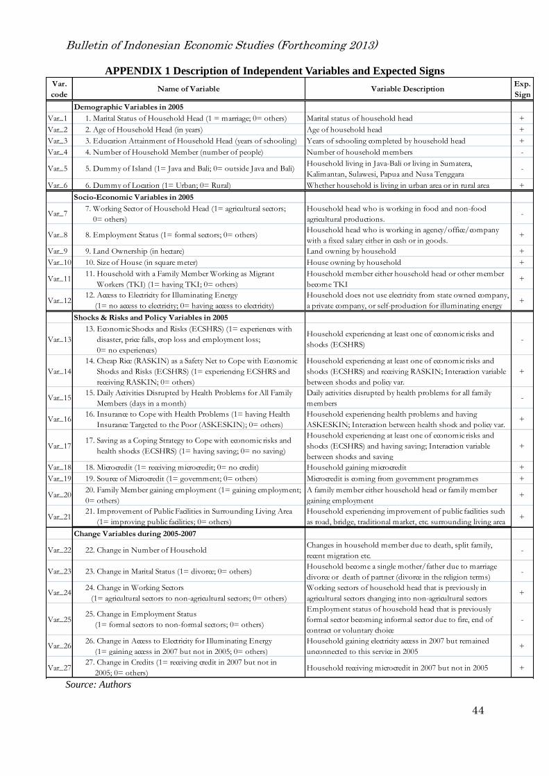
Bulletin of Indonesian Economic Studies (Forthcoming 2013)
44
APPENDIX 1 Description of Independent Variables and Expected Signs
Demographic Variables in 2005
Var_1 1. Marital Status of Household Head (1 = marriage; 0= others) Marital status of household head +
Var_2 2. Age of Household Head (in years) Age of household head +
Var_3 3. Education Attainment of Household Head (years of schooling) Years of schooling completed by household head +
Var_4 4. Number of Household Member (number of people) Number of household members -
Var_5 5. Dummy of Island (1= Java and Bali; 0= outside Java and Bali)Household living in Java-Bali or living in Sumatera,
Kalimantan, Sulawesi, Papua and Nusa Tenggara-
Var_6 6. Dummy of Location (1= Urban; 0= Rural) Whether household is living in urban area or in rural area +
Socio-Economic Variables in 2005
Var_77. Working Sector of Household Head (1= agricultural sectors;
0= others)
Household head who is working in food and non-food
agricultural productions.-
Var_8 8. Employment Status (1= formal sectors; 0= others)Household head who is working in agency/office/company
with a fixed salary either in cash or in goods.+
Var_9 9. Land Ownership (in hectare) Land owning by household +
Var_10 10. Size of House (in square meter) House owning by household +
Var_1111. Household with a Family Member Working as Migrant
Workers (TKI) (1= having TKI; 0= others)
Household member either household head or other member
become TKI+
Var_1212. Access to Electricity for Illuminating Energy
(1= no access to electricity; 0= having access to electricity)
Household does not use electricity from state owned company,
a private company, or self-production for illuminating energy+
Shocks & Risks and Policy Variables in 2005
Var_13
13. Economic Shocks and Risks (ECSHRS) (1= experiences with
disaster, price falls, crop loss and employment loss;
0= no experiences)
Household experiencing at least one of economic risks and
shocks (ECSHRS)-
Var_14
14. Cheap Rice (RASKIN) as a Safety Net to Cope with Economic
Shocks and Risks (ECSHRS) (1= experiencing ECSHRS and
receiving RASKIN; 0= others)
Household experiencing at least one of economic risks and
shocks (ECSHRS) and receiving RASKIN; Interaction variable
between shocks and policy var.
+
Var_1515. Daily Activities Disrupted by Health Problems for All Family
Members (days in a month)
Daily activities disrupted by health problems for all family
members-
Var_1616. Insurance to Cope with Health Problems (1= having Health
Insurance Targeted to the Poor (ASKESKIN); 0= others)
Household experiencing health problems and having
ASKESKIN; Interaction between health shock and policy var.+
Var_1717. Saving as a Coping Strategy to Cope with economic risks and
health shocks (ECSHRS) (1= having saving; 0= no saving)
Household experiencing at least one of economic risks and
shocks (ECSHRS) and having saving; Interaction variable
between shocks and saving
+
Var_18 18. Microcredit (1= receiving microcredit; 0= no credit) Household gaining microcredit +
Var_19 19. Source of Microcredit (1= government; 0= others) Microcredit is coming from government programmes +
Var_2020. Family Member gaining employment (1= gaining employment;
0= others)
A family member either household head or family member
gaining employment+
Var_2121. Improvement of Public Facilities in Surrounding Living Area
(1= improving public facilities; 0= others)
Household experiencing improvement of public facilities such
as road, bridge, traditional market, etc. surrounding living area+
Change Variables during 2005-2007
Var_22 22. Change in Number of HouseholdChanges in household member due to death, split family,
recent migration etc.-
Var_23 23. Change in Marital Status (1= divorce; 0= others)Household become a single mother/father due to marriage
divorce or death of partner (divorce in the religion terms)-
Var_2424. Change in Working Sectors
(1= agricultural sectors to non-agricultural sectors; 0= others)
Working sectors of household head that is previously in
agricultural sectors changing into non-agricultural sectors+
Var_2525. Change in Employment Status
(1= formal sectors to non-formal sectors; 0= others)
Employment status of household head that is previously
formal sector becoming informal sector due to fire, end of
contract or voluntary choice
-
Var_2626. Change in Access to Electricity for Illuminating Energy
(1= gaining access in 2007 but not in 2005; 0= others)
Household gaining electricity access in 2007 but remained
unconnected to this service in 2005+
Var_2727. Change in Credits (1= receiving credit in 2007 but not in
2005; 0= others)Household receiving microcredit in 2007 but not in 2005 +
Name of Variable Variable DescriptionExp.
Sign
Var.
code
Source: Authors
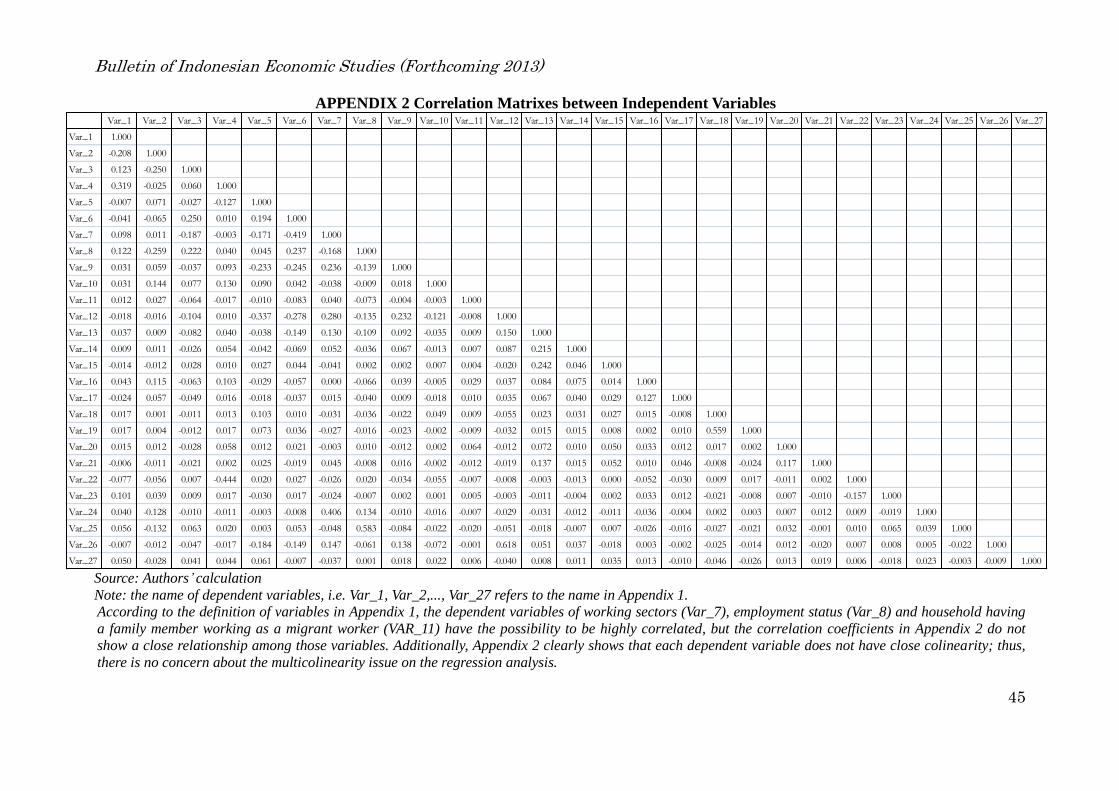
Bulletin of Indonesian Economic Studies (Forthcoming 2013)
45
APPENDIX 2 Correlation Matrixes between Independent Variables Var_1 Var_2 Var_3 Var_4 Var_5 Var_6 Var_7 Var_8 Var_9 Var_10 Var_11 Var_12 Var_13 Var_14 Var_15 Var_16 Var_17 Var_18 Var_19 Var_20 Var_21 Var_22 Var_23 Var_24 Var_25 Var_26 Var_27
Var_1 1.000
Var_2 -0.208 1.000
Var_3 0.123 -0.250 1.000
Var_4 0.319 -0.025 0.060 1.000
Var_5 -0.007 0.071 -0.027 -0.127 1.000
Var_6 -0.041 -0.065 0.250 0.010 0.194 1.000
Var_7 0.098 0.011 -0.187 -0.003 -0.171 -0.419 1.000
Var_8 0.122 -0.259 0.222 0.040 0.045 0.237 -0.168 1.000
Var_9 0.031 0.059 -0.037 0.093 -0.233 -0.245 0.236 -0.139 1.000
Var_10 0.031 0.144 0.077 0.130 0.090 0.042 -0.038 -0.009 0.018 1.000
Var_11 0.012 0.027 -0.064 -0.017 -0.010 -0.083 0.040 -0.073 -0.004 -0.003 1.000
Var_12 -0.018 -0.016 -0.104 0.010 -0.337 -0.278 0.280 -0.135 0.232 -0.121 -0.008 1.000
Var_13 0.037 0.009 -0.082 0.040 -0.038 -0.149 0.130 -0.109 0.092 -0.035 0.009 0.150 1.000
Var_14 0.009 0.011 -0.026 0.054 -0.042 -0.069 0.052 -0.036 0.067 -0.013 0.007 0.087 0.215 1.000
Var_15 -0.014 -0.012 0.028 0.010 0.027 0.044 -0.041 0.002 0.002 0.007 0.004 -0.020 0.242 0.046 1.000
Var_16 0.043 0.115 -0.063 0.103 -0.029 -0.057 0.000 -0.066 0.039 -0.005 0.029 0.037 0.084 0.075 0.014 1.000
Var_17 -0.024 0.057 -0.049 0.016 -0.018 -0.037 0.015 -0.040 0.009 -0.018 0.010 0.035 0.067 0.040 0.029 0.127 1.000
Var_18 0.017 0.001 -0.011 0.013 0.103 0.010 -0.031 -0.036 -0.022 0.049 0.009 -0.055 0.023 0.031 0.027 0.015 -0.008 1.000
Var_19 0.017 0.004 -0.012 0.017 0.073 0.036 -0.027 -0.016 -0.023 -0.002 -0.009 -0.032 0.015 0.015 0.008 0.002 0.010 0.559 1.000
Var_20 0.015 0.012 -0.028 0.058 0.012 0.021 -0.003 0.010 -0.012 0.002 0.064 -0.012 0.072 0.010 0.050 0.033 0.012 0.017 0.002 1.000
Var_21 -0.006 -0.011 -0.021 0.002 0.025 -0.019 0.045 -0.008 0.016 -0.002 -0.012 -0.019 0.137 0.015 0.052 0.010 0.046 -0.008 -0.024 0.117 1.000
Var_22 -0.077 -0.056 0.007 -0.444 0.020 0.027 -0.026 0.020 -0.034 -0.055 -0.007 -0.008 -0.003 -0.013 0.000 -0.052 -0.030 0.009 0.017 -0.011 0.002 1.000
Var_23 0.101 0.039 0.009 0.017 -0.030 0.017 -0.024 -0.007 0.002 0.001 0.005 -0.003 -0.011 -0.004 0.002 0.033 0.012 -0.021 -0.008 0.007 -0.010 -0.157 1.000
Var_24 0.040 -0.128 -0.010 -0.011 -0.003 -0.008 0.406 0.134 -0.010 -0.016 -0.007 -0.029 -0.031 -0.012 -0.011 -0.036 -0.004 0.002 0.003 0.007 0.012 0.009 -0.019 1.000
Var_25 0.056 -0.132 0.063 0.020 0.003 0.053 -0.048 0.583 -0.084 -0.022 -0.020 -0.051 -0.018 -0.007 0.007 -0.026 -0.016 -0.027 -0.021 0.032 -0.001 0.010 0.065 0.039 1.000
Var_26 -0.007 -0.012 -0.047 -0.017 -0.184 -0.149 0.147 -0.061 0.138 -0.072 -0.001 0.618 0.051 0.037 -0.018 0.003 -0.002 -0.025 -0.014 0.012 -0.020 0.007 0.008 0.005 -0.022 1.000
Var_27 0.050 -0.028 0.041 0.044 0.061 -0.007 -0.037 0.001 0.018 0.022 0.006 -0.040 0.008 0.011 0.035 0.013 -0.010 -0.046 -0.026 0.013 0.019 0.006 -0.018 0.023 -0.003 -0.009 1.000
Source: Authors’ calculation
Note: the name of dependent variables, i.e. Var_1, Var_2,..., Var_27 refers to the name in Appendix 1.
According to the definition of variables in Appendix 1, the dependent variables of working sectors (Var_7), employment status (Var_8) and household having
a family member working as a migrant worker (VAR_11) have the possibility to be highly correlated, but the correlation coefficients in Appendix 2 do not
show a close relationship among those variables. Additionally, Appendix 2 clearly shows that each dependent variable does not have close colinearity; thus,
there is no concern about the multicolinearity issue on the regression analysis.