UNIVERSITI PUTRA MALAYSIA

SIMULATIONS OF ONSET OF CONVECTION IN A NON·NEWTONIAN LIQUID INDUCED BY UNSTEADY·STATE HEAT CONDUCTION

TING KEE CHIEN

FK 2001 23

SIMULATIONS OF ONSET OF CONVECTION IN A NON·NEWTONIAN LIQUID INDUCED BY UNSTEADY·STATE HEAT CONDUCTION

By

TING KEE CHIEN

Thesis Submitted in Fulfilment of the Requirement for the Degree of Master of Science in the Faculty of Engineering

Universiti Putra Malaysia

December 200t

Abstract of thesis presented to the Senate of Universiti Putra Malaysia in fulfilment of the requirement for the degree of Master of Science

SIMULATIONS OF ONSET OF CONVECTION IN A NON-NEWTONIAN LIQUID INDUCED BY UNSTEADY-STATE HEAT CONDUCTION

By

TING KEE CHIEN

December 2001

Chairman: Associate Professor Tan Ka Kheng, Ph.D.

Faculty : Engineering

The onset of convection in an initially static non·Newtonian liquid under Fixed

Surface Temperature (FST) and Constant Heat Flux (CHF) boundary conditions was

simulated using a CFD package. Steady-state and unsteady-state simulations were

successfully conducted for bottom surface heating of shear thinning non·Newtonian

liquids. Simulations on Newtonian liquid water and glycerine were conducted to

verify the simulation setup.

Fourier's law of heat conduction was used to validate the steady-state simulation

results. Simulations conducted for non·Newtonian liquid with Tien et al.'s (1969)

experimental data were found to agree well with Fourier's law at conduction phase.

Tien et al.'s definition of non-Newtonian power-law Rayleigh number was found to

be inadequate in representing the onset of convection in non-Newtonian liquid.

Attempts to determine the Rayleigh number for non-Newtonian liquid using

apparent viscosity was successfully carried out. A more realistic critical Rayleigh

number for non-Newtonian liquid was successfully determined with local values of

Rayleigh number around a convection cell successfully obtained.

For simulations conducted for unsteady-state heat conduction in non·Newtonian

liquid, transient heat conduction theory was used to validate the results. Convection

was found to occur in a continuous deep fluid bounded by two horizontal rigid

surfaces and adiabatic vertical walls. Transient critical Rayleigh number for non­

Newtonian liquid under unsteady state heat conduction defined by Tan (1994) was

successfully applied. Transient critical Rayleigh number for non-Newtonian liquid

was found to vary with flow behavior n of the Power Law model. A more realistic

transient critical Rayleigh number for non-Newtonian liquid was successfully

determined using apparent viscosity.

Development of thermal plumes in viscous non-Newtonian liquid were found to

differ slightly from the development of thermal plumes in non-viscous Newtonian

liquid. The NumBx for unsteady-state simulations of Newtonian and non-Newtonian

liquid were observed to be 3.8 ± 2.0 for FST cases and 2.7 ± 1.8 for CHF cases.

Effect of boundary condition at interface on onset of transient convection were

studied. Velocity boundary condition of a top surface solid were found to be best

approximated using top-cooling simulations. Bottom-heating simulations in a deep

fluid revealed that the upper interface boundary has the property between a solid and

a free surface.

ii

Abstrak tesis yang dikemukakan kepada Senat Universiti Putra Malaysia sebagai memenuhi keperluan untuk ijazah Master Sains

SIMULASI PERMULAAN PEROLAKAN DALAM CECAIR DUKAN NEWTONIAN YANG DIARUm KONDUKSI DADA TIDAK MANTAP

Oleh

TING KEE CHIEN

Disem ber 2001

Pengerusi: Professor Madya Tan Ka Kheng, Ph.D.

Faculti : Kejuruteraan

PermuJaan peroJakan daJam cecair bukan Newtonian yang statik pada muJanya di

bawah keadaan Permukaan Suhu Tetap (FST) dan Fluks Haba Tetap (CHF) telah

disimulasikan dengan pakej Pengiraan Dinamik Bendalir (CFD). Simulasi untuk

keadaan mantap dan keadaan tidak mantap telah berjaya dilaksanakan untuk

pemanasan cecair bukan Newtonian dari permukaan bawah. Simulasi ke atas cecair

Newtonian air dan glycerine telah dilaksanakan untuk mengesahkan penetapan

simulasi.

Teori konduksi haba Fourier telah digunakan dalam pemastian keputusan untuk

simuJasi keadaan mantap. SimuJasi yang dilaksanakan untuk cecair bukan

Newtonian dengan data ujikaji Tien et al. (1969) telah didapati mematuhi teori

Fourier dengan baiknya pada fasa konduksi. Definisi Tien et al. untuk nombor

Rayleigh cecair bukan Newtonian power-law telah didapati kurang memuaskan

dalam pengambaraan permulaan perolakan di dalam cecair bukan Newtonian

Percubaan untuk menentukan nombor Rayleigh untuk cecair bukan Newtonian

dengan menggunakan kepekatan ketara telah berjaya dilakukan. Suatu nombor

Rayleigh untuk cecair bukan Newtonian yang lebih realistik telah betjaya ditentukan

jii

dengan nilai tempatan nombor Rayleigh di sekitar satu sel perolakan berjaya

didapati.

Untuk simulasi yang dilaksanakan untuk konduksi haba tidak mantap di dalam

cecair bukan Newtonian, teoTi konduksi haba tidak mantap teJah digunakan dalam

pemastian keputusan simulasi. Perolakaan dapat diperhatikan di dalam cecair

berlanjutan dibatasi dua sempadan mendatar yang tegar dan dua dinding tegak

adiabatik. Nombor Rayleigh kritikal tidak mantap bagi cecair bukan Newtonian

yang didefinisikan oleh Tan (1994) untuk konduksi haba tidak mantap telah berjaya

digunakan. Nombor Rayleigh kritikal tidak mantap bagi cecair bukan Newtonian

didapati berubah dengan indeks sifat pengaliran cecair n dalam model Power Law.

Suatu nombor Rayleigh tidak mantap untuk cecair bukan Newtonian yang lebih

realistik telah berjaya ditentukan dengan menggunakan kelikatan ketara.

Perubahan kepulan haba di dalam cecair bukan Newtonian pekat didapati berlainan

sedikit dengan perubahan di dalam cecair Newtonian yang cairo Numax untuk

simulasi keadaan tidak mantap cecair Newtonian dan cecair bukan Newtonian

didapati berada dalam lingkungan 3.8 ± 2.0 untuk kes-kes FST dan 2.7 ± 1.8 untuk

kes-kes CHF.

Kesan keadaan sempadan di permukaan dwihala pada permulaan perolakaan telah

diselidiki. Keadaan sempadan halaju yang tegar pada permukaan atas didapati

paling baik dikaji dengan simulasi penyejukan dari atas. Simulasi pemanasan dari

bawah dalam cecair berJanjutan mencadangkan permukaan dwihala atas mempunyai

sifat di antara tegar dan tidak tegar.

iv

ACKNOWLEDGEMENTS

The author wishes to express his deepest gratitude to his supervisors, Associate

Professor Dr. Tan Ka Kheng of Chemical and Environmental Engineering

Department, Dr. Thomas Choong of Chemical and Environmental Engineering

Department, Mr. Hishammuddin bin Jamaluddin of Biological and Agricultural

Engineering Department and Dr. Nor Mariah Adam of Mechanical and

Manufacturing Engineering Department for their invaluable advice and guidance

throughout the course of this subject.

The proVISIOn of a scholarship by the Ministry of Science, Technology and

Environment under National Science Fellowship scheme IS gratefully

acknowledged.

The spiritual support and encouragement given by family members and friends have

carried the author through the struggles of materializing this thesis.

v

I certify that an Examination Committee met on 1 ih November 2001 to conduct the final examination of Ting Kee Chien on his Master of Science thesis entitled "Simulations of Onset of Convection in Non-Newtonian Liquids Induced by Unsteady-State Heat Conduction" in accordance with Universiti Pertanian Malaysia (Higher Degree) Act 1980 and Universiti Pertanian Malaysia (Higher Degree) Regulations 1981. The Committee recommends that the candidate be awarded the relevant degree. Members of the Examination Committee are as follows:

DA YANG RADIAH A WANG BIAK, Ph.D.

Department of Chemical and Environmental Engineering Faculty of Engineering Universiti Putra Malaysia (Chairperson)

TAN KA KHENG, Ph.D.

Associate Professor Department of Chemical and Environmental Engineering Faculty of Engineering Universiti Putra Malaysia (Member)

THOMAS CHOONG SHEAN YAW, Ph.D.

Department of Chemical and Environmental Engineering Faculty of Engineering Universiti Putra Malaysia (Member)

HISHAMMUDDIN BIN JAMALUDIN, M.Sc.

Department of Biological and Agricultural Engineering Faculty of Engineering Universiti Putra Malaysia (Member)

NOR MARIAH ADAM, Ph.D.

Associate Professor Department of Mechanical and Manufacturing Engineering Universiti Putra Malaysia (Member)

AINI IDERIS, Ph. D.,

ProfessorlDean of Graduate School, Universiti Putra Malaysia

Date:'1 7 JAN 2002

vi

This thesis submitted to the Senate of Universiti Putra MaJaysia has been accepted as fulfilment of the requirement for the degree of Master of Science.

AINI IDERIS, Ph. D. Professor, Dean of Graduate School, Universiti Putra Malaysia

Date: 1 4 MAR 2002

vii

DECLARATION

I hereby declare that the thesis is based on my original work except for quotations and citations which have been duly acknowledged. I also declare that it has not been previously or concurrently submitted for any other degree at UPM or other institutions.

Ting Kee Chien �'"

Date: '""1 jllt\.,..a"l 2002,.

viii

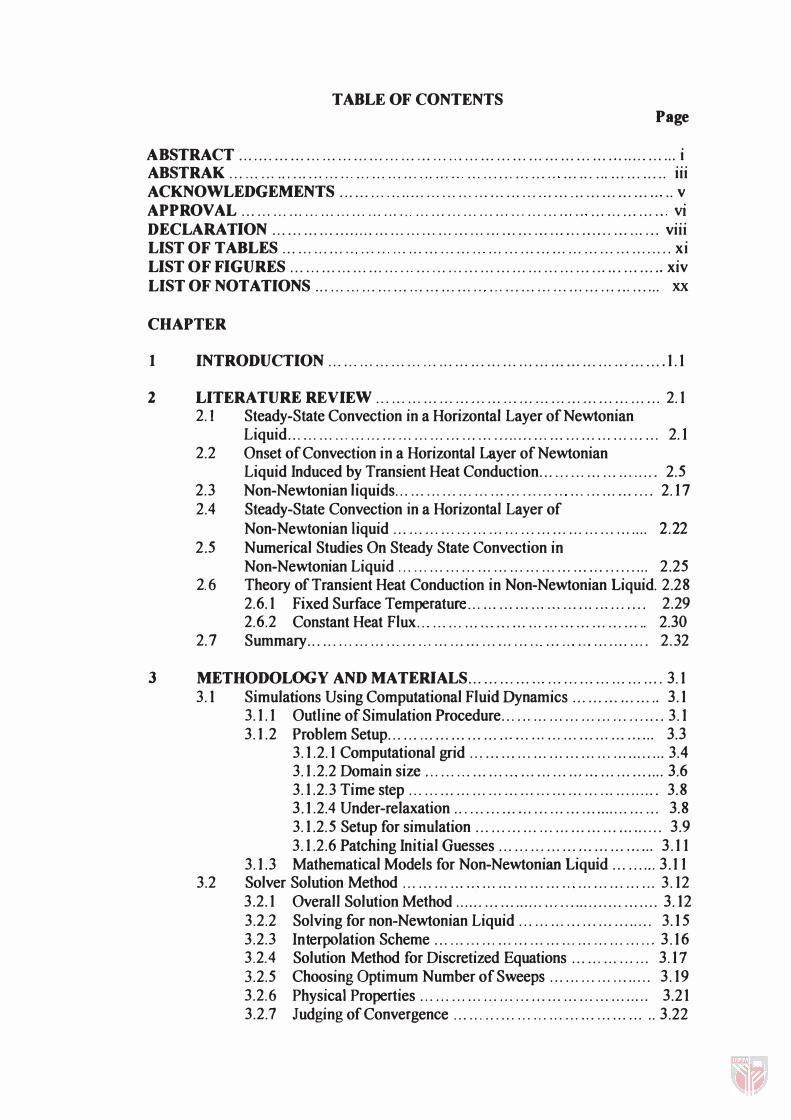
TABLE OF CONTENTS Page

ABSTRACT . . . . . . . . . . . . . . . . . . . . . . . . . . . . . . . . . . . . . . . . . . . . . . . . . . . . . . . . . . . . . . . . . . . . . . . . . . . . . . . . . . . . i ABSTRAK . . . . . . . . , .. , ..... , .. . '" ... ... . , . ... ... .. , '" ., ....... . , ... . '" .. , ... ... ... ... ... .. iii ACKNOWLEDGEMENTS . . . . . . . .. ... . . . . . . .. . . . . . ... . . . . . . . . . . . . . . . . . . . . . . . . . . . . ... '" .. v APPROVAL . . . . . , ... . , . ...... ...... ... .. , '" ., . ............ '" .. , ... ... '" '" .. , ... ..... , '" vi DECLARATION . . . . . . . . . . . . . . . . . . . . . . . . . . . . . . . . . . . . . . . . . . . , ... ......... ......... ... ...... viii LIST OF TABLES . . . . . . . . . . . . '" . . , '" .. .. .. ... .. . ... '" ... ......... ... ... ...... .. , ........ xi LIST OF FIGURES . . . . . . . . . . . . . . . . . . . . . '" .... .. .. ... , ... ...... .............. , ... ... ... .. xiv LIST OF NOTATIONS . . . . . . . . . . . . . . . . . . . . . . . . . . . . . . '" .. , ... ... .. , ... . " ... ... ... .. . ... xx

CHAPTER

1 INTRODUCTION . . . . .. . . . . . . . .. . . . .. . . . , ... . .... ..... , . .. . . . . . . , .. . . . . . . , . . . . . . . 1.1

2 LITERATURE REVIEW . . . . . . . . . . . . . . . . . . . . . . . . . . . . . . .. . . . . . . , ... . . . . . . . .. . .. 2. 1 2.1 Steady-State Convection in a Horizontal Layer of Newtonian

Liquid . . . . . . . . . . . . . . . . . . . . . . . . . . . . . . . . . . . . . . . . . . . . . . . . . . . . . . . . . . . . . . . . . . . . . . . 2.1 2.2 Onset of Convection in a Horizontal Layer of Newtonian

Liquid Induced by Transient Heat Conduction . . . .. . . . . . . . . . . . . , .. . . , 2.5 2.3 Non-Newtonian liquids . . . . . . . . . . . . . .. . . . . . , ......... '" ... ... .. . . . . .... 2.1 7 2.4 Steady-State Convection in a Horizontal Layer of

Non-Newtonian liquid . . . . . . .. . . . . . . . . . . . . . . . . . . . . . . . . . . . . . . . . . . . . . . . . . 2.22 2.5 Numerical Studies On Steady State Convection in

Non-Newtonian Liquid . . . . .. .. . . . . ... .. . .. . . . . . .. ... .. . .. . . .. ......... 2. 25 2.6 Theory of Transient Heat Conduction in Non-Newtonian Liquid. 2.28

2.6.1 Fixed Surface Temperature .. . . . . . . , . .. '" ." ... . .. .. , ... . . . . 2. 29 2.6.2 Constant Heat Flux . . . . . . . . . . . . . . . . " . . . . .. . .. '" . . . .. . .. . . . . .. 2.30

2.7 Summary . . . . . . . . . . . . . . . . . . . .. .. , ... ... . . . ... . .. ... '" . . , '" '" .. . ... . .. . . 2.32

3 METHODOLOGY AND MATERIALS .. . . . . . . . . . . '" . . . .. . . .. . . . .. . . . . . . .. 3. 1 3.1 Simulations Using Computational Fluid Dynamics . . . . . . .. . . . . . . . . . 3.1

3.1. 1 Outline of Simulation Procedure . . . . . , .. . ...... ... . . , .. . .... . . . 3.1 3. 1.2 Problem Setup . . . . . . . . , . . . . . . .. , ... '" ... '" . . . . . . . . . . . , . . . . ,. . . . 3. 3

3.1.2.1 Computational grid . . , . . . . " .. . . . . . .. . .. . . . .. . . . . . . ... . . . 3.4 3.1.2.2 Domain size . . . . . . . . . . " . .. '" . .. . .. ... . . . '" . . . .. . '" ... . 3.6 3.1. 2.3 Time step . . . . . . . . . . . . . . . . . . . . . . . , ... ... .. . .. ... . . .. ..... . 3. 8 3.1.2.4 Under-relaxation ... .. . . . . . . . ... . . . ... .. . .. . . . . .. .. .. . ... 3. 8 3.1.2. 5 Setup for simulation . .. . . . . . . . .. . . . . . . . . . . . . . . . . ... . . . . . 3.9 3.1. 2.6 Patching Initial Guesses . . . . . . .. . . . . . . . . . . .. . . . .. . . ... 3.11

3.1. 3 Mathematical Models for Non-Newtonian Liquid . . . . . . . . . 3.11 3.2 Solver Solution Method . . . . . , . . . . . . '" . .. . . . ... .. . . . . '" ... . . . .. . .. . . .. 3.12

3. 2.1 Overall Solution Method . . . . . . . . . . . . . . . . . . . . . . . . .. . . . . . . .. . . . . . . . 3. 12 3.2.2 Solving for non-Newtonian Liquid . . . . . . . . . . . . . . . . .... . . . . . . 3.15 3.2.3 Interpolation Scheme . . . . . . . . . . . . . . . . . . . . . . . . . . . . . . . . . . . . . . . . . . 3.16 3.2.4 Solution Method for Discretized Equations . . . . . . . . . . . . . . . 3.17 3.2.5 Choosing Optimum Number of Sweeps . . . . .. . . . . . . . . . . . . . . 3.19 3.2.6 Physical Properties . . . . . . . . . . .. . . . . . . . . . . . . . . . . . . . . . . . . . . . ... .. 3. 21 3.2.7 Judging of Convergence . . . . . .. . . . . . . . . .. . . . . . . . . . . . . . .. . . . . .. 3.22

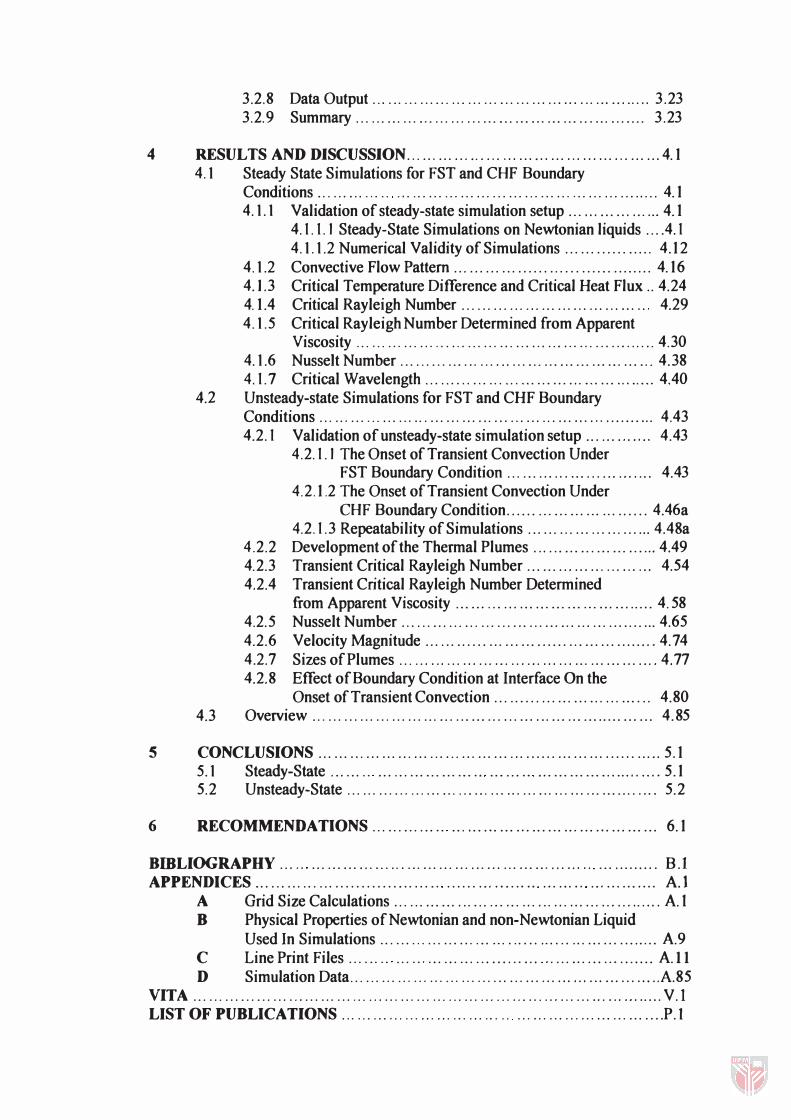
3.2.8 Data Output . . . . . . . . . . . . . . . . . . . . . . . . . . . . . . . . .. . . . . . . . . . .. . .. . . . . . 3.23 3. 2.9 Summary . . . . . . . . . . . . .. . . . . . . . . . . . .. .. . . .. ... . . . . . . . . . .. .. . . . . . . 3.23

4 RESULTS AND DiSCUSSiON ...... ... ......... ... ...... ... ... ......... ... .. . 4. 1 4.1 Steady State Simulations for FST and CHF Boundary

Conditions .......... , . '" . , . . . . . . . . . . . . . . . . . . . . . . . . . . . . ... . . . . . . . . . . . . . . . . . 4. 1 4.1.1 Validation of steady-state simulation setup .. . . . . ... .. . ... . . . 4.1

4.1. 1. 1 Steady-State Simulations on Newtonian liquids .. . . 4.1 4.1.1.2 Numerical Validity of Simulations ................. 4.12

4.1.2 Convective Flow Pattern ...................................... 4. 16 4.].3 Critical Temperature Difference and Critical Heat Flux .. 4. 24 4.1.4 Critical Rayleigh Number . . . .. . . . . .. . . . . . . . . . , .. . . .. .. . . . . '" 4. 29

4.1.5 Critical Rayleigh Number Determined from Apparent Viscosity . . . . . . '" . . . . . ..... " ... . . . ... ... ... . .. .. , .. . . . . . . . . . .... 4. 30

4.1.6 Nussett Number ... . . . . . . . . . . . . . . . . . . . . . ... ... .. . . . .. ........ ... 4.38 4.1.7 Critical Wavelength . .. ..... ... . . .. . .. . ... ..... .. ... . . ... . , . .. .. 4.40

4.2 Unsteady-state Simulations for FST and CHF Boundary Conditions . . . . .. . . . .. , .. . . . . ... ... ... ... ...... . . . ... ... .. . '" ." .......... 4. 43 4.2.1 Validation of unsteady-state simulation setup ... . . . . . . . . .. 4.43

4. 2. 1. 1 The Onset of Transient Convection Under FST Boundary Condition . . . . . . . . . . . . .. . . . . . .. . .. . .. . 4.43

4.2.1.2 The Onset of Transient Convection Under CHF Boundary Condition ........................... 4.46a

4. 2.1. 3 Repeatability of Simulations ........................ 4.48a 4. 2.2 Development of the Thermal Plumes . . . . . . .. . .. . . . . .. . . . . .. . 4.49 4. 2.3 Transient Critical Rayleigh Number... . . . ... .. . .. . . . . . . . . .. 4. 54 4.2.4 Transient Critical Rayleigh Number Determined

from Apparent Viscosity ... . . . . . . . . . .... .. . .. .. . . .. . .. . . . . . . . . 4.58 4.2.5 Nusselt Number ........... , . . . . . . . . . . .. . . .. .. ..... . . . . . . . . . . . . .. 4.65 4.2.6 Velocity Magnitude ............................................ 4.74 4.2.7 Sizes of Plumes . . . . . . . . . . . . . . . . .. .. . . . . . . . . . . . . .. . . . . .. .. . .. ... . 4.77 4.2.8 Effect of Boundary Condition at Interface On the

Onset of Transient Convection .............................. 4. 80 4.3 Overview . .. . . . . . . . . . . . . . . . . . . . . ... . . .. . ... . . . . .. .. . . . .. . .. . .. . .. .. . . . . . . . 4.85

5 CONCLUSIONS ... ... ...... ... .................. ...... ...... ......... ...... ..... 5 .1 5.1 Steady-State ...... ' " .. . .. . .. .. . , .. . ... ' " . . . . . . ' " . . . . . . . . . . . . .. . . .. .... . , 5 . 1 5.2 Unsteady-State . . . . . . . . . . .. . . . .. . .. . . . . . .. . . .. . . . . .. . .. .. . . . . . . .. .. . . . . . .. 5.2

6 RECOMMENDATIONS . . . . . .. . . ... '" . . , .. . . , . . . . . , . . . .... .. , ... . , . . .. .. . .. . 6.1

BmLIOGRAPHY . . . '" ............. , .................................... , '" ., .......... B.l APPENDICES .. . . . . . . . . . . . , . .............. , ... '" ...... ........ , '" ., . ... '" ... ... ....... A.I

A Grid Size Calculations . . . . . . . .. ... . . . ... . .. .. . . . . . . . . . . . ... . .. . . ... .. . . . . At

B Physical Properties of Newtonian and non-Newtonian Liquid Used In Simulations ..................................................... A9

C Line Print Files . . . . . . '" ... '" ... ... ... ... ..... , ......... . , .... .......... All

D Simulation Data . . . . . . . .. . . , ... . .. .. . . .. .. . . .. .. . ... . .. .. . ... ... ........... A.85 VITA . . . . . . . . . . . . . . . . . . . . . . . . . . . . . . . . . . . . . . . . . . . . . . . . . . . . . . . . . . . . . . . . . . . . . . . . . . . . . . . . . . . . .. . . . V.l LIST OF PUBLICATIONS . .. . . . . . . '" .................. '" ...... ...................... P.I

LIST OF TABLES

TABLE

2.1. The critical Rayleigh numbers and wave numbers for various Biot

Page

numbers and physical boundary conditions. (Sparrow et al., 1964) ., . . ... 2.11

2.2. Equations of maximum transient Rae for various boundary conditions. (Tan & Thorpe, 1999) ... ... .... , . . . .. ... . , .... . . .. ... .. , . .. . . .. . . . ... ... .. .. . . . . 2. 12

2.3 Equations used for predicting the sizes of plumes under various boundary conditions. (Tan & Thorpe, t 999b) . ... .. . ... .. ... ... . .. '" .. . . . . . .2.16

2.4 Flow behavior n and correlating constants. (Tan, 1994) . . . . . . . . .. . . . . . . . . . 2. 31

3.1 Problem setup for 2-D steady-state simulations . . . . . . . . .. ... ... .. . . . . . . . . . . . 3. 24

3.2 Problem setup for 2-D unsteady-state simulations . ... .. . . .. . . . . . .. . . . . , . . ... 3.25

4. I . Summary of steady state heat conduction simulation runs conducted for Newtonian and non-Newtonian liquid under FST and CHF boundary conditions . .. , ... ... ........ , ... .... . . .. . . , . .. . . . . ... '" ... . . . .. . . , . .. . . 4. 2

4. 2. A comparison of theoretical, experimental and simulated ATe for Newtonian liquid under steady-state FST bottom-heating boundary condition . . , . .. . ... .... . . . , . ... . . . . , . .. . .... . . . .. . . . . . . . . . . .. . . . . . . . . , . . . . , . . . . . . . .. . 4. 4

4.3. A comparison of theoretical and simulated le for Newtonian liquid under steady-state CHF bottom-heating boundary condition . . . . .... 4. 4

4. 4. Simulation results of steady-state glycerine conducted with and without gravitational force under CHF boundary condition . . .. .. , . .. .. . . . . 4. 12

4. 5. A comparison of ATe predicted using Tien et al.'s model, experiment and simulation for non-Newtonian liquid under steady-state FST bottom-heating boundary condition . . . . . .. . . . .. . . . . . . . . . . . . . .. . . .. . . . ... . .. .. . 4. 26

4.6. A comparison of ATe predicted using Tien et al.'s model with RGNN = 1708, experiment and simulation for non-Newtonian liquid under steady-state FST bottom-heating boundary condition . . . . '" '" .. .. 4.27

4.7. A comparison of ATs predicted using Tien et al.'s model and simulation for non-Newtonian liquid under steady-state CHF bottom-heating boundary condition . . . . . .. .. .... . . . ... .. . . . . . . . . . . ... . . . .. . . . . 4.27

4.8. A comparison of ATs predicted using Tien et al.'s model with RaNN = 1296 and simulation for non-Newtonian liquid under steady-state CHF bottom-heating boundary condition . . . . . . . . , . . . . . .. ... '" 4. 27

xi

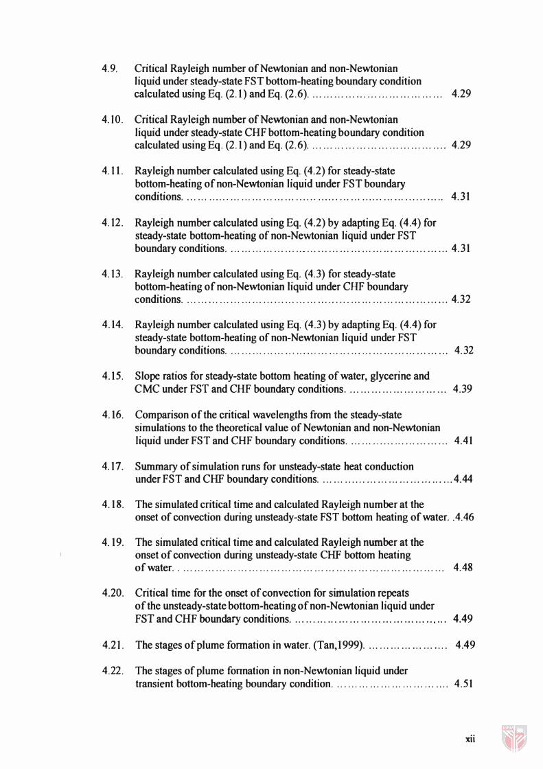
4.9. Critical Rayleigh number of Newtonian and non-Newtonian liquid under steady-state FST bottom-heating boundary condition calculated using Eq. (2.1) and Eq. (2.6). ... ... ... . .. ... ... ... ... ... .. . ... ... 4.29

4.10. Critical Rayleigh number of Newtonian and non-Newtonian liquid under steady-state CHF bottom-heating boundary condition calculated using Eq. (2.1) and Eq. (2.6) . ... ......... ............... ... ... .... 4.29

4.11. Rayleigh number calculated using Eq. (4.2) for steady-state bottom-heating of non-Newtonian liquid under FST boundary conditions .... . . , ..... , ... .. , . .. ... ...... ..... , ..... , ... .. , ..... , . .. .. , ..... , .... . 4.31

4.12. Rayleigh number calculated using Eq. (4.2) by adapting Eq. (4. 4) for steady-state bottom-heating of non-Newtonian liquid under FST boundary conditions. .. . .. , .. . .. , ...... '" .. , ...... ... .. , .. . ... ... .. , ...... ... .. , 4.31

4. 13. Rayleigh number calculated using Eq. (4.3) for steady-state bottom-heating of non-Newtonian liquid under CHF boundary conditions . ... .................. ............ ... ........... , ... ... ... . .. ..... . ...... 4.32

4.14. Rayleigh number calculated using Eq. (4. 3) by adapting Eq. (4.4) for steady-state bottom-heating of non-Newtonian liquid under FST boundary conditions . ............... ........ , ... ............... ..... , ...... .. .... 4.32

4.15. Slope ratios for steady-state bottom heating of water, glycerine and CMC under FST and CHF boundary conditions . ............ ... . ....... .... 4.39

4.16. Comparison of the critical wavelengths from the steady-state simulations to the theoretical value of Newtonian and non-Newtonian liquid under FST and CHF boundary conditions . .. . . .. ......... . .. ... ...... 4.41

4.17. Summary of simulation runs for unsteady-state heat conduction under FST and CHF boundary conditions . . .... . ...... ... ... . .. .. . ... ...... .. .4.44

4.18. The simulated critical time and calculated Rayleigh number at the onset of convection during unsteady-state FST bottom heating of water, .4.46

4.19. The simulated critical time and calculated Rayleigh number at the onset of convection during unsteady-state CHF bottom heating of water. . . . . . . . . . . . . . . . . . . . . . . . . . . . . . . . . . . . . . . . . . . . . . . . . . . . . . . . . . . . . . . . . . . . . . . . . . 4.48

4.20. Critical time for the onset of convection for simulation repeats of the unsteady-state bottom-heating of non-Newtonian liquid under FST and CHF boundary conditions . ... ......... .... .. ...... ... ... ...... '" ... 4.49

4.21. The stages of plume formation in water. (Tan, 1999). ... .. . .. . ...... ... . ... 4.49

4.22. The stages of plume fonnation in non-Newtonian liquid under transient bottom-heating boundary condition . .... .... . .. . ... . .. . , . ... . , . .... 4.51

xii

4.23. Simulated critical times and critical transient Rayleigh Numbers for bottom heating of glycerine and non-Newtonian liquid under FST boundary condition . ........ , ..... , ..... , ... ... ... ... ... ... .. , ... .. , ... ...... ... 4.54

4.24. Simulated critical times and critical tmnsient Rayleigh Numbers for bottom heating of glycerine and non-Newtonian liquid under CHF boundary condition. ... ......... ... ... ... ......... ... ... .. , ." ... .. , ... ... ... ... 4.55

4.25. Critical Rayleigh number calculated using Eq. (4.7) for unsteady-state bottom-heating of non-Newtonian liquid under FST boundary conditions . ......... ...... .... , . ..... , ......... ......... . , . ......... .. , 4.59

4.26. Critical Rayleigh number calculated using Eq. (4.8) for unsteady-state bottom-heating of non-Newtonian liquid under CHF boundary conditions. ... ......... ... ... ... ... ... ............ ......... ... ......... 4.59

4.27. Equations used to calculated Nusselt Number for FST and CHF boundary condition. (Sam, 1999)... ............... ...... ... ... ... ...... ....... 4.65

4.28. Maximum Nusselt number Numax for Newtonian and non-Newtonian liquids obtained from simulation results under FST boundary condItion . .................. ... ... ...... ... ...... ...... . " ........... , ... ... ... .... 4.68

4.29. Maximum Nusselt number Numax for Newtonian and non-Newtonian liquids obtained from simulation results under CHF boundary condition . . . . . . . . . . . . . . . . . . . . . . . . . . . . . . . . . . . . . . . . . . . . . . . . . . . . . . . . . . . . . . . . . . . . . . . . . .. 4.68

4.30. Comparison of the critical wavelength A.c from the unsteady-state simulations to the predicted value of Newtonian and non-Newtonian liquid under FST boundary conditions Table 2.3 and Eq. (2.13) respectively . .................. ..... , .................. ... . .. .... . .. ......... '" ... 4.78

4.31. Comparison of the critical wavelength A.c from the unsteady-state simulations to the predicted value of Newtonian and non-Newtonian liquid under CHF boundary conditions Table 2.3 and Eq. (2.17) respectively . ... ............ ... ... ......... ...... ...... . , . ..... , ... ... ....... ... ... 4.78

4.32. Critical Rayleigh number for various boundary conditions. (Tan & Thorpe, 1999b) ...... ......... ... ... ......... ...... ...... ............... 4.81

4.33. Critical Rayleigh number for various heat conduction mode and boundary conditions in a liquid layer. (Tan & Thorpe, 1999b) ...... ..... , 4.81

4.34. A comparison of the critical time for onset of convection and Rayleigh number for Newtonian and non-Newtonian liquid under unsteady-state FST bottom-heating and top-cooling boundary condition . ...... '" ........ 4.82

4.3 5. A comparison of the critical time for onset of convection and Rayleigh number for Newtonian liquid under unsteady-state CHF top-cooling and bottom-heating boundary condition . ......... ...... ... ... ...................... 4.83

xiii

LIST OF FIGURES

FIGURE Page

2.1. A typical Schmidt & Milverton's graph showing the discontinuity in the rate of heat transfer in a layer of fluid between two horizontal plates when heated from below. Photographs taken at times corresponding to the indicated points of (a) to (e) are shown in Figure 2.2. (Schmidt & Milverton, 1935) . .. ... . .. ... ..... , ...... ....... ...... 2.3

2.2. Photographs showing the changes of heat transfer mode from conduction to convection in a layer of fluid between two horizontal plates when heated from below, which was taken at the screen at times corresponding to the indicated points in Figure 2.1. (a) No heating current being passed. (b) A temperature gradient has been established but the stability point has not been reached. (c) The instability point has now been passed, and it is seen that the band has widened and its upper edge has become wavy. (d) The upper edge of the image is deflected farther from the zero position on account of the greater heat transfer. (e) The heat transfer is now greater still, and the motion correspondingly violent. (Schmidt & Milverton, 1935) ......... . , .... ... .. , . 2.4

2.3. Uneven surface layer observed just before the onset of convection during the transient evaporative cooling of water. (Spangenberg & Rowland, 1961) .... .. ..... . ... .... .. ... ... '" ......... ... ... .. . 2.5

2.4. Top view and front view of simultaneous sheet and columnar plunging in water during the start of transient top-cooling convective circulation. Inverted plumes can be observed at the front view. (Spangenberg & Rowland, 1961) . ........ .. .... ......... ......... . 2.6

2.5. Convection cells observed during the transient evaporative cooling of water. (Foster, 1965b) . .. .... .. ... ... ..... . ......... ...... ... ...... ... ... ... .. 2.8

2.6. Thermals rising in water as a result of unsteady-state heat introduced at the bottom surface. Photograph below showed thermals that formed at a lower heating rate. (Sparrow et al., 1970) ... ... ... ..... . ... .... 2.9

2.7. The development of the thermal plumes from 60s to 130 s for cooling of water under CHF boundary conditions. (Tan, 1999) ......... 2.13

2.8. Relationship between shear stress and velocity gradient for Newtonian liquid and non-Newtonian liquid . . . , ... '" . . , ... . , .... ...... ... .... ... .... , . ... 2.18

2.9. A typical log f.J versus log i' graph showing variation of viscosity with

shear rate for a non-Newtonian liquid . . . . .. .. .. . .... . .... ..... ...... ... ... .... 2.19

2.10. A typical set of data by Tien et al. showing the best-fit line for steady-state conduction and convection respectively in non-Newtonian liquid. (Tien et aI., 1969) ... ... ............... ...... ... ...... 2.23

x.iv

2. 1 J . Predicted value and experimental results of the critical Rayleigh number RaNNc versus the flow behavior index n, as reported by Tien et al (1969) . .................... , . .. ... ...... ...... ... .... .. ... '" ., . .. . . ... 2.24

2.12. Sequence of instabilities in viscoelastic Rayleigh-Benard convection under steady-state heat conduction. (a) Ra = 2268. (b) Ra = 2745 (a) Ra = 3180 (d) Ra = 7226 (e) Ra = 24375 (f) Ra = 31088 (g) Ra = 56884 (h) Ra = 76113 (i) Ra = 208686 Gampert & Domjahn, 1989) ... ... ... ... ... ... ... ...... ... ... ... ........... ... 2.26

2.13. Series of differential interferograms in silicone oil. At Ra = 24000, the non-linear vertical heat conduction profile is replaced by convective instabilities. (Zierep & Oertel 1982) ... ......... ...... ... ... '" ... ... ... ..... 2.27

3.1. Boundary conditions for steady-state and unsteady-state bottom heating simulations of a liquid . .. . . . . . " ... . " .. , .. . ... ... ... ... ... .. . ... ... ... 3.3

3.2. The thickness of non-Newtonian liquid. (a) Finite depth for steady-state heat conduction (b) Penetration depth for unsteady-state heat conduction . . . . . . . . . . . . . . . . . . . . . . . . . . . . . . . . . . . . . . . . . . . . . . . . . . . . . . . . . . . . . . . . . . . . 3.4

3.3. Impact of the near-wall grid spacing on the shear stress calculation in laminar flow. (a) Grid spacing I1n too large. (b) Better grid spacing An . . . 3.6

3.4. Overview of the solution process . . .. .. . ... ... .. ...... ....... ... ...... ... ... ... 3.1 4

3.5. Typical computational cell surrounding node P . . . . .. .. . .. . . . . . .. . .. ... .. . .. . 3.16

3.6. (a): Illustration of J(y) sweep direction. (b) Illustration of l(x) sweep direction. . . . ...... ......... ... ...... ... ... ... ... ....... " ... ... ... ... ... ... 3.19

3.7. Alternating direction sweeps by FLUENT during simulations. ........... 3.20

3.8. Multiple sweeps for the pressure equation . . . . . . . . .. .. . ... . .. .. . .. . . . . . . . ... . 3.21

4.1. Heat flux versus temperature difference for bottom heating of water under steady-state FST boundary condition . . . . ... ... . . , '" ... .. , ... '" .. , ... 4.2

4.2 Heat flux versus surface temperature difference for bottom heating of water under steady-state CHF boundary condition . . . . . .. . . , ... ... .. , ... ... 4.5

4.3. Steady-state bottom-heating of water under FST boundary condition with AT= lK. (a) Temperature contour (b) Velocity vector . . . ... ... ... .. 4.6

4.4. Steady-state bottom-heating of water under FST boundary condition with I1T= 4K. (a) Temperature contour (b) Velocity vector . . . . . . . ,. ..... 4.7

4.5. Steady-state bottom-heating of water under FST boundary condition with I1T= 10K. (a) Temperature contour (b) Velocity vector . . . . . . . . . . . . 4.8

xv

4.6. Steady-state bottom-heating of water under CHF boundary condition with l= 40W/m2. (a) Temperature contour (b) Velocity vector.. . ... ... 4.9

4.7. Steady-state bottom-heating of water under CHF boundary condition with qO= 200W/m2. (a) Temperature contour (b) Velocity vector... .... 4.10

4.8. Steady-state bottom-heating of water under CHF boundary condition with l= 800W/m2. (a) Temperature contour (b) Velocity vector... ... . 4.11

4.9. Temperature contour for steady-state bottom-heating of glycerine under CHF boundary condition with l = 100W/m2 and without gravitational force . ... '" . .. ... ........ . ...... .. ..... . , ... '" .... , .... '" '" . .. ... . , . ... .. , .... ... 4.13

4.10. Temperature contour for steady-state bottom-heating of glycerine under CHF boundary condition with l = 200W/m2 and without gravitational force . ... ... ....... , ......... ........... .. '" ............ . . , '" ... ......... ........ 4.13

4.11. Steady-state bottom-heating of glycerine under CHF boundary condition with l = 100W/m2 and gravitational force. (a) Temperature contour (b) Stream function .. .... .. ........... ..... ... ... 4.14

4.12. Steady-state bottom-heating of glycerine under CHF boundary condition with l = 200W/m2 and gravitational force. (a) Temperature contour (b) Stream function ... ... ... . , ... , .. , ... .. . .... , . 4.15

4. 13. Steady-state bottom-heating of non-Newtonian liquid CMC-5 (n = 0.94) under FST boundary condition with I1T= 2K. (a) Temperature contour (b) Velocity vector ... .. , . .. '" ....... , . ......... ... 4.18

4.14. Steady-state bottom-heating of non-Newtonian liquid CMC-5 (n = 0. 94) under FST boundary condition with I1T= 4K. (a) Temperature contour (b) Velocity vector ... .. , ...... .... , . ... ...... ... ... 4.19

4.15. Steady-state bottom-heating of non-Newtonian liquid CMC-5 (n = 0.94) under FST boundary condition with 111'= 6K. (a) Temperature contour (b) Velocity vectoT. ..... .. . ... . .. ... .. , '" ... ... . , . 4.20

4.16. Steady-state bottom-heating of non-Newtonian liguid CMC-5 (n = 0.94) under CHF boundary condition with qO= 100W/m2. (a) Temperature contour (b) Velocity vector ... ... ........ ...... ...... . , . .... 4.21

4.17. Steady-state bottom-heating of non-Newtonian liquid CMC-5 (n = 0.94) under CHF boundary condition with l= 150W/m2. (a) Temperature contour (b) Velocity vector ., . .. , '" '" ... . .. ... ... '" ...... 4.22

4. 18. Steady-state bottom-heating of non-Newtonian liquid CMC-5 (n = 0.94) under CHF boundary condition with l= 300W/m2. (a) Temperature contour (b) Velocity vector .. , ... '" ... .... , .... '" '" .... 4.23

xvi

4.1 9. Heat flux versus temperature difference for bottom heating of non-Newtonian liquid CMC-7 (n = 0.70; d= 0.02667m) under steady-state FST boundary condition . ...... ... . , ... , ...... '" ., . .. , ... ....... 4.28

4.20. Heat flux versus surface temperature difference for bottom heating of non-Newtonian liquid CMC-7 (n = 0.70; d= 0. 02667m) under steady-state CHF boundary condition . .... .. ... ... '" ... ......... ... .. , ... ... 4.28

4.21. Critical Rayleigh number calculated using Eq. (4.2) versus n for steady-state simulations of non-Newtonian liquid under FST boundary condition. ... ... ... ... ... ... ... ... ... ... ... ... ... ... ... ... ... ... ... ... 4.34

4.22. Critical Rayleigh number calculated using Eq. (4.3) versus n for steady-state simulations of non-Newtonian liquid under CHF boundary condition . ......... ...... ...... ... ...... ...... ....... ....... , ...... ... 4.34

4.23. Rayleigh numbers before convection occurs in a steady-state bottom-heating simulation for non-Newtonian liquid (n = 0.70) under FST boundary condition .... ... . , ............. ... ... .... ...... , ... , ...... 4.35

4.24. Rayleigh numbers around a convection cell in a steady-state bottom-heating simulation for non-Newtonian liquid (n = 0.70) under FST boundary condition . ..... . ... ... .... ..... ... ... . .. . .. . .. . ... . . ... ... 4.35

4.25. Rayleigh numbers before convection occurs in a steady-state bottom-heating simulation for non-Newtonian liquid (n = 0.70) under CHF boundary condition . ... ... ... ...... ... ... ....... ..... ... ...... ..... 4.37

4.26. Rayleigh numbers around a convection cell in a steady-state bottom-heating simulation for non-Newtonian liquid (n = 0.70) under CHF boundary condition . ... .. . . , . ... . .. ... '" ., . .. , '" ....... , . ... ..... 4.37

4.27. Steady-state Nu versus n for Newtonian and non-Newtonian liquid under FST and CHF boundary conditions . .. ............. ... ... ... .... . . ..... 4.40

4.28. Comparison of the critical wavelength predicted by the theory for Newtonian liquid and the observed value for non-Newtonian liquid under steady-state FST boundary condition . ... . , . .. , ... ... ........ .... ..... 4.42

4.29. Comparison of the critical wavelength predicted by the theory for Newtonian liquid and the observed value for non-Newtonian liquid under steady-state CHF boundary condition . ........ . ... ... '" ., . ........... 4.42

4.30. Theoretical and simulated total heat conduction into water versus square root time under FST boundary condition when .1T=O.5K. ........ 4.45

4.30a. Theoretical and simulated total heat conduction into non-Newtonian liquid (CMC-2; n = 0.877; .1T= 25K) versus square root time under FST boundary condition . ...... ...... '" ...... ... '" '" ...... ...... ..... 4.46a

xvii

4. 31. Theoretical and simulated heat transfer coefficient of water versus time under CHF boundary condition when l=100W/m2

. • . . • . , . • . • . . . . . . 4.47a

4. 31a. Theoretical and simulated heat transfer coefficient of non· Newtonian liquid versus time under CHF boundary condition (CMC-2� n = 0.877� qO = 2000W/m2). . ..... ... '" . .. .. . . . . ... .. . . . . .. . . ... .. . 4.48

4. 32. The development stages of thennal plumes in non-Newtonian liquid (CMC-I; n = 1.006) under unsteady·state FST bottom-heating boundary condition . . ... . . . . .. .. , .. . ... ... . .. . . . '" . .. .. . . .. . . . . . . . . . . . . . . . .. . . . . . .. .. . . . . 4. 52

4. 33. The development stages of thennal plumes in non-Newtonian liquid (CMC-4; n = 0. 45) under unsteady-state FST bottom-heating boundary condition . . . . .. . '" '" ... . . . .. . ... . .. . ..... ... . .. . .. . .. ... '" .. . ... . . . . . . .. . . .. . . . 4. 53

4. 34. RaNNc versus n for non-Newtonian liquid under FST boundary condition . . . . . ... ... '" ... ... . . . .. . ... ... . . , ... .. . .. . ... .. . ... . . . . . . ... . .. . .. . .. .. . 4.56

4.35. RaNNc versus n for non-Newtonian liquid under CHF boundary condition. ... ... ... .. . . . . . . . . . . ... . .. .. . ... . .. . .. . . . ... .. . ... ... .. . . . . . .. ... ... . . . 4.56

4. 36 Unsteady-state bottom-heating of non-Newtonian liquid (n = 0. 85) under FST boundary condition. (a) Temperature contour (b) Velocity vector (c) Apparent viscosity . . . . .. . . .. .... . . . . . . . . . .. . .. . .... . . .. ... . . . ... ... .. 4.62

4. 37 Unsteady-state bottom-heating of non-Newtonian liquid (n = 0.94) under CHF boundary condition. (a) Temperature contour (b) Velocity vector (c) Apparent viscosity . ... ... . .. .. . . . . .. . . . . ... .. ... . .. . .. . ... . . . .. . ... . . 4. 63

4.38. Transient critical Rayleigh number calculated using Eq. (4.7) versus n for unsteady-state simulations of non-Newtonian liquid under FST boundary condition . . .. . . . . . . .. . . . . . . . . . . . . . . . , ......... ...... ... ... ............. 4.64

4. 39. Transient critical Rayleigh number calculated using Eq. (4.8) versus n for unsteady-state simulations of non-Newtonian liquid under CHF boundary condition . . . . . . . . . . . . . . . . . . . . . . . . . . . . . . . . . . . . . . . . . . . . . . . . . . . . . . . . . . . . . . 4. 64

4. 40. T ota} heat conducted versus square root time for transient bottom heating of Newtonian liquid under FST boundary condition (water� &T= O.5K). .. .. . .. .. . ... . . . . . . ...... ... .. . .. . . .. ......... ......... ... ... 4.69

4. 4 I . NusseIt number versus time for transient bottom heating of Newtonian liquid under FST boundary condition (water; &T= 0.5K) . . .. . . . .. . ... . .. . 4.69

4.42. Total heat conducted versus square root time for transient bottom heating of non-Newtonian liquid under FST boundary condition (CMC-2; n = 0.877; &T= 25K) . . . . . . .. .. , . . . . . . . . . . . . .. . . . . . .. . . . . . . . . . .. ... .. . 4. 70

xviii

4.43. Nusselt number versus time for tmnsient bottom heating of non-Newtonian liquid under FST boundary condition (CMC-2; n = 0.877; AT = 25K) . . . . . . . . . . . . , . . . . . . . . . . . . . . . . . . . . . . . . . . . , . . . . . . . 4.70

4.44. Heat tmnsfer coefficient versus time for transient bottom heating of Newtonian liquid under eHF boundary condition (water; l = 100W/m2). . . . .. . . . . . . . . , . . . , . . . . . . . , . . . . . . . . . . . . . . . . . . . ' " . , . . . . . . . 4 .71

4.45. Nusselt number versus time for tmnsient bottom heating of Newtonian liquid under CHF boundary condition (water; l = 100W/m2) . .. . . . . . . . . . . . 4.71

4.46. Heat tmnsfer coefficient versus time for tmnsient bottom heating of non-Newtonian liquid under CHF boundary condition (CMC-2; n = 0.877; qO = 2000W/m2) . . . . . , . . . . . . . . . . . , . . . , . . . ' " . , . . . . . . . . ' " 4.72

4.47. Nusselt number versus time for tmnsient bottom heating of non-Newtonian liquid under CHF boundary condition (CMC-2; n = 0.877; l = 2000W/m2) . . . . . . . . . . ' " . . . . . .. . .. . . . , . . . . . . . . . .. . . . . 4.72

4.48. NumBx versus n for transient bottom heating of non-Newtonian liquid under FST boundary condition. ' " . , . . . . . . . . . . . , . . . , . . . . . . . . . . . . . . . .. . . . . . . . . . . 4.73

4.49. NumBx versus n for transient bottom heating of non-Newtonian liquid under CHF boundary condition . . . . .. . . . . . . . . . . . . . ' " . .. . . . . . . . . . . . . . . . . . . . . . . . . 4.73

4.50. Maximum velocity magnitude for transient bottom-heating of non-Newtonian l iquid CMC-2 (n = 0.877) under FST boundary condition . . . . . . . . . . . , . . . . .. . , . . . , . . . . . . . , . . . . ' " . . . . . . . . , . . . . . . . . . . . , . . . . ' " . . . . . . . . 4.75

4.51. Maximum velocity magnitude for transient bottom-heating of non-Newtonian liquid CMC-2 (n = 0.877) under CHF boundary condition . . . . . . . . . . . . . . . . .. , . . . . , . . . . .. . . . . . . . . . . . . . . . . . , . . . . . . . . . . . . . . . , . . . . . . . . . . 4.76

4.52. Comparison of the theoretical and simulated critical wavelengths for Newtonian and non-Newtonian liquids under unsteady-state FST boundary condition calculated using equations from Table 2.3 and Eq. (2. 13) respectively . . . . . . . . . . . . . . . . . . . . . . . . . . . . . . . ' " . , . . . , . . . . . . . . . . . , . . . . . . . 4.79

4.53. Comparison of the theoretical and simulated critical wavelengths for Newtonian and non-Newtonian liquids under unsteady-state CHF boundary condition calculated using equations from Table 2.3 and Eq. (2. 17) respectively . . . . . . . . . . . . . . . . . . . . . . . . , . . . . . . . . . . . . . . . . . . . . . . . . . . . . . . . . . . 4.79

xix

LIST OF NOTATIONS

ac Dimensionless wave number

B Constant rate of surface temperature variation (K/s)

C Heating current (A)

cp Specific heat (J/kg.K)

D Diameter (m)

d Total depth of liquid layer for steady-state heat conduction (m)

g Gravitational acceleration (m/s2)

h Heat transfer coefficient (W/m2.K)

k Thermal conductivity (W/m. K)

K Consistency index (Pa.sn)

I Liquid depth for unsteady-state heat conduction (m)

n Flow behaviour index in Power Law model

Nu Nusselt number

q Heat flux (W/m2)

l Constant surface heat flux (W/m2)

q Total heat conducted per area into the liquid (J/m2)

Q Heat input (W)

Ra Rayleigh number

RONNe Critical transient Rayleigh number for non-Newtonian liquid

Pe Peclet number

t Time (s)

T Temperature (K)

�T Temperature difference between top and bottom surfaces (K)

xx

u Fluid velocity (m/s)

X Horizontal length of computational domain (m)

Ax Computational grid size in horizontal direction (m)

Y Vertical height of computational domain (m)

L\y Computational grid size in vertical direction (m)

z Vertical distance in liquid measured from the bounding surface (m)

Greek Symbols

a Volumetric coefficient of thermal expansion (K-1)

P (Constant) temperature gradient (Klm)� p = L\T / d

8 Thickness of effective thermal layer (m)

r ratio of thermal conductivity to heat capacity (kgls.m)� r = k I cp

i' Strain rate (S-I)

1( Thermal diffusivity (m2/s)

A Wavelength (m)

Ji Viscosity (Pa.s)

Jlapp Apparent Viscosity (Pa.s)

v Kinematic Viscosity (m2/s)

p Density (kglm3)

u Under relaxation factor

xxi

Subscripts

c Critical

0 Initial state

s Surface

T temperature dependent

app apparent

max Maximum

Abbreviation

CFD Computational Fluid Dynamics

CHF Constant Heat Flux

CMC Carboxy Methyl Celulose

FST Fixed surface temperature

NN Non-Newtonian liquid

xxii

CHAPTER 1

INTRODUCTION

Studies of natural convection phenomena have been done in general for many years

in natural sciences like astrophysics, geology, oceanography, climatology and

meteorology. In convection, the hotter and lighter fluid rises while the colder and

heavier fluid sinks. Natural convection, or free convection, seems to have been first

described by Thomson ( 1 882), but the first quantitative experiment was done by

Benard ( 1 900).

Lord Rayleigh ( 1 9 16) studied the onset of buoyancy convection in a horizontal

liquid layer bounded by two free surfaces based on an adverse linear temperature

gradient. A dimensionless stability parameter was defined after him, the Rayleigh

number. Convection occurs when Rayleigh number exceeded its critical value.

For natura1 convection induced by a time-dependent and non-linear temperature

profile, Tan and Thorpe ( 1 996) developed a new transient Rayleigh number for the

deep fluid under various boundary conditions. They proposed that the correct way

to begin any stability analysis is to identify the Biot number. They analyzed

previous researchers' experimental data by first determine the Biot number for each

case (Tan & Thorpe, 1 996; 1 999a). Critical Rayleigh number were re-calculated

and found to be consistent within a range of identified Biot number and wave

number.

1 . 1